import numpy as np
import pandas as pd

import matplotlib.pyplot as plt

pd.set_option('display.max_columns', None)Practical 9: Dimensionality reduction
This week, we will focus on conducting dimensionality reduction on the performance and disadvantage variables of schools in England, trying to understand which variables (or variable combinations) are important in distinguishing these schools.
We will use the method of principal component analysis (PCA).
Dataset
We’re going to use the filtered school data that has been used in previous practicals.
# read in the dataset from Github
df_school = pd.read_csv("https://raw.githubusercontent.com/huanfachen/QM/refs/heads/main/sessions/L6_data/Performancetables_130242/2022-2023/england_filtered.csv")
Check the shape and columns of this data frame.
print(f"df_school has {df_school.shape[0]} rows and {df_school.shape[1]} columns.")
print("First 5 rows:\n")
print(df_school.head(5))
df_school has 3056 rows and 37 columns.
First 5 rows:
URN SCHNAME.x LEA LANAME TOWN.x \
0 100053 Acland Burghley School 202 Camden London
1 100054 The Camden School for Girls 202 Camden London
2 100052 Hampstead School 202 Camden London
3 100049 Haverstock School 202 Camden London
4 100059 La Sainte Union Catholic Secondary School 202 Camden London
gor_name TOTPUPS ATT8SCR ATT8SCRENG ATT8SCRMAT ATT8SCR_FSM6CLA1A \
0 London 1163.0 50.3 10.7 10.2 34.8
1 London 1047.0 65.8 13.5 12.7 54.7
2 London 1319.0 44.6 9.7 9.1 39.3
3 London 982.0 41.7 8.7 8.8 37.7
4 London 817.0 49.6 10.8 9.4 45.9
ATT8SCR_NFSM6CLA1A ATT8SCR_BOYS ATT8SCR_GIRLS P8MEA P8MEA_FSM6CLA1A \
0 59.2 51.5 46.8 -0.16 -0.99
1 72.0 NaN 65.8 0.77 0.25
2 49.0 41.9 47.1 -0.03 -0.18
3 48.5 40.1 43.7 -0.28 -0.44
4 52.2 NaN 49.6 0.06 -0.20
P8MEA_NFSM6CLA1A PTFSM6CLA1A PTNOTFSM6CLA1A PNUMEAL PNUMENGFL \
0 0.34 37.0 63.0 23.6 70.5
1 1.13 36.0 64.0 25.5 73.7
2 0.09 45.0 55.0 38.1 61.9
3 0.02 63.0 37.0 57.5 41.9
4 0.25 41.0 59.0 50.6 46.0
PTPRIORLO PTPRIORHI NORB NORG PNUMFSMEVER PERCTOT PPERSABS10 \
0 15.0 33.0 765.0 398.0 39.6 8.1 24.7
1 5.0 50.0 139.0 908.0 30.3 4.5 6.6
2 21.0 18.0 681.0 638.0 51.3 8.2 24.0
3 30.0 15.0 559.0 423.0 69.8 10.1 33.1
4 16.0 28.0 40.0 777.0 42.7 10.3 33.8
SCHOOLTYPE.x RELCHAR ADMPOL.y ADMPOL_PT \
0 State-funded secondary Does not apply Non-selective OTHER NON SEL
1 State-funded secondary NaN Non-selective OTHER NON SEL
2 State-funded secondary Does not apply Non-selective OTHER NON SEL
3 State-funded secondary Does not apply Non-selective OTHER NON SEL
4 State-funded secondary Roman Catholic Non-selective OTHER NON SEL
gender_name OFSTEDRATING MINORGROUP easting northing
0 Mixed Good Maintained school 528962.0 185931.0
1 Girls Good Maintained school 529441.0 184659.0
2 Mixed Good Maintained school 524402.0 185633.0
3 Mixed Good Maintained school 528159.0 184498.0
4 Girls Good Maintained school 528379.0 186191.0 The metadata of this data is available here. For convenience, the columns are described as below:
1. URN: Unique Reference Number identifying a school.
2. SCHNAME.x: School name as recorded in the official register.
3. LEA: Local Education Authority (code).
4. LANAME: Name of the Local Authority.
5. TOWN.x: Town in which the school is located.
6. gor_name: Government Office Region name.
7. TOTPUPS: Total number of pupils on roll.
8. ATT8SCR: Average Attainment 8 score for all pupils.
9. ATT8SCRENG: Average Attainment 8 score for English subject grouping.
10. ATT8SCRMAT: Average Attainment 8 score for Maths subject grouping.
11. ATT8SCR_FSM6CLA1A: Average Attainment 8 score for pupils eligible for Free School Meals in the last 6 years and/or Children Looked After.
12. ATT8SCR_NFSM6CLA1A: Average Attainment 8 score for pupils not eligible for Free School Meals in the last 6 years and not Children Looked After.
13. ATT8SCR_BOYS: Average Attainment 8 score for male pupils.
14. ATT8SCR_GIRLS: Average Attainment 8 score for female pupils.
15. P8MEA: Progress 8 measure for all pupils.
16. P8MEA_FSM6CLA1A: Progress 8 measure for disadvantaged pupils (FSM6 and/or CLA1A).
17. P8MEA_NFSM6CLA1A: Progress 8 measure for non-disadvantaged pupils.
18. PTFSM6CLA1A: Percentage of pupils eligible for FSM6 and/or CLA1A.
19. PTNOTFSM6CLA1A: Percentage of pupils not eligible for FSM6 and/or CLA1A.
20. PNUMEAL: Percentage of pupils whose first language is known or believed to be other than English.
21. PNUMENGFL: Percentage of pupils whose first language is English.
22. PTPRIORLO: Percentage of pupils with low prior attainment from Key Stage 2.
23. PTPRIORHI: Percentage of pupils with high prior attainment from Key Stage 2.
24. NORB: Number of boys on roll.
25. NORG: Number of girls on roll.
26. PNUMFSMEVER: Percentage of pupils who have been eligible for free school meals in the past six years (FSM6 measure).
27. PERCTOT: Percentage of total pupil absence (authorised and unauthorised combined).
28. PPERSABS10: Percentage of pupils who are persistently absent (overall absence rate 10% or more).
29. SCHOOLTYPE.x: Official classification of the school type (e.g., Academy, Community, Voluntary Aided).
30. RELCHAR: Religious character of the school (e.g., Church of England, Roman Catholic, None).
31. ADMPOL.y: Admission policy type (e.g., non-selective, selective).
32. ADMPOL_PT: Percentage breakdown related to admission policy (context-specific).
33. gender_name: Gender intake of the school (Mixed, Boys, Girls).
34. OFSTEDRATING: Latest Ofsted inspection overall effectiveness grade.
35. MINORGROUP: Ethnic minority group classification for aggregation purposes.
36. easting: Ordnance Survey Easting coordinate of school location.
37. northing: Ordnance Survey Northing coordinate of school location.
As the focus is to explore the performance and disadvantage ratio of schools, we will keep the following variables:
- PTFSM6CLA1A – Percentage of pupils eligible for Free School Meals in the past six years (FSM6) and/or Children Looked After (CLA1A).
- PTNOTFSM6CLA1A – Percentage of pupils not eligible for FSM6 and not CLA1A.
- PNUMEAL – Percentage of pupils whose first language is known or believed to be other than English.
- PNUMFSMEVER – Percentage of pupils who have ever been eligible for Free School Meals in the past six years (FSM6 measure).
- ATT8SCR_FSM6CLA1A – Average Attainment 8 score for pupils eligible for FSM6 and/or CLA1A.
- ATT8SCR_NFSM6CLA1A – Average Attainment 8 score for pupils not eligible for FSM6 and not CLA1A.
- ATT8SCR_BOYS – Average Attainment 8 score for male pupils.
- ATT8SCR_GIRLS – Average Attainment 8 score for female pupils.
- P8MEA_FSM6CLA1A – Progress 8 measure for disadvantaged pupils (FSM6 and/or CLA1A).
- P8MEA_NFSM6CLA1A – Progress 8 measure for non-disadvantaged pupils.
Please note - we remove the count variables (e.g. NORB and NORG), as the count variables are affected by the pupil size of each school. We also remove variables that are redundant due to perfect correlation with those retained, such as PNUMENGFL, which is equal to 1-PNUMEAL.
# Extract the selected columns
df_school_reduced = df_school[
    [
        'PTFSM6CLA1A', 'PTNOTFSM6CLA1A', 'PNUMEAL', 'PNUMFSMEVER',
        'ATT8SCR_FSM6CLA1A', 'ATT8SCR_NFSM6CLA1A', 'ATT8SCR_BOYS', 'ATT8SCR_GIRLS',
        'P8MEA_FSM6CLA1A', 'P8MEA_NFSM6CLA1A'
    ]
]

# Display the first few rows
print(df_school_reduced.head())
PTFSM6CLA1A PTNOTFSM6CLA1A PNUMEAL PNUMFSMEVER ATT8SCR_FSM6CLA1A \
0 37.0 63.0 23.6 39.6 34.8
1 36.0 64.0 25.5 30.3 54.7
2 45.0 55.0 38.1 51.3 39.3
3 63.0 37.0 57.5 69.8 37.7
4 41.0 59.0 50.6 42.7 45.9
ATT8SCR_NFSM6CLA1A ATT8SCR_BOYS ATT8SCR_GIRLS P8MEA_FSM6CLA1A \
0 59.2 51.5 46.8 -0.99
1 72.0 NaN 65.8 0.25
2 49.0 41.9 47.1 -0.18
3 48.5 40.1 43.7 -0.44
4 52.2 NaN 49.6 -0.20
P8MEA_NFSM6CLA1A
0 0.34
1 1.13
2 0.09
3 0.02
4 0.25 Task one: to address missing values and to standardise variables
We expect that all variabels in df_school_reduced are of numerical type. It is safe to check it before further analysis.
print("Numeric columns: {}".format(df_school_reduced.select_dtypes(include='number').columns.tolist()))
print("Non-numeric columns: {}".format(df_school_reduced.select_dtypes(exclude='number').columns.tolist()))
Numeric columns: ['PTFSM6CLA1A', 'PTNOTFSM6CLA1A', 'PNUMEAL', 'PNUMFSMEVER', 'ATT8SCR_FSM6CLA1A', 'ATT8SCR_NFSM6CLA1A', 'ATT8SCR_BOYS', 'ATT8SCR_GIRLS', 'P8MEA_FSM6CLA1A', 'P8MEA_NFSM6CLA1A']
Non-numeric columns: []To convert all columns to numeric, we can use the following code. Note that numeric columns are not affected.
df_school_reduced = df_school_reduced.apply(pd.to_numeric, errors='coerce')Now, let’s check whether our dataset has any missing values — this is important because PCA in sklearn package cannot handle NaN values directly.
To display the number of missing entries for each column:
# Check missing values column by column
missing_counts = df_school_reduced.isnull().sum()
print("Missing values per column:\n", missing_counts)
Missing values per column:
PTFSM6CLA1A 86
PTNOTFSM6CLA1A 86
PNUMEAL 25
PNUMFSMEVER 25
ATT8SCR_FSM6CLA1A 128
ATT8SCR_NFSM6CLA1A 126
ATT8SCR_BOYS 294
ATT8SCR_GIRLS 244
P8MEA_FSM6CLA1A 138
P8MEA_NFSM6CLA1A 131
dtype: int64
Note
There are two common ways to deal with missing values:
- Remove all rows with at least one missing values. In this dataset, this leads to loss of many rows (around 10%).
- Impute the missing values using a selected imputation method.
To fill in these missing values, we will use the KNNImputer() from sklearn.impute.
This method finds the k closest rows (neighbors) to the one with the missing value and uses their values to compute an average for imputation.
It’s a smarter approach than simply filling with the mean or median because it considers patterns across all variables.
from sklearn.impute import KNNImputer

# Create our KNN imputer (k=5 is a common choice, but can be tuned)
imputer = KNNImputer(n_neighbors=5)

# Fit to our data and transform it
df_school_reduced = pd.DataFrame(
    imputer.fit_transform(df_school_reduced),
    columns=df_school_reduced.columns,  # Keep original column names
    index=df_school_reduced.index       # Keep original index
)

# Double-check that there are no more missing values
print("Are all missing values handled?:", df_school_reduced.isnull().sum().sum() == 0)
Are all missing values handled?: TrueThen, we will compare all variables in terms of their range, mean, and variance.
df_school_reduced.describe()| PTFSM6CLA1A | PTNOTFSM6CLA1A | PNUMEAL | PNUMFSMEVER | ATT8SCR_FSM6CLA1A | ATT8SCR_NFSM6CLA1A | ATT8SCR_BOYS | ATT8SCR_GIRLS | P8MEA_FSM6CLA1A | P8MEA_NFSM6CLA1A | |
|---|---|---|---|---|---|---|---|---|---|---|
| count | 3056.000000 | 3056.000000 | 3056.000000 | 3056.000000 | 3056.000000 | 3056.000000 | 3056.000000 | 3056.000000 | 3056.000000 | 3056.000000 |
| mean | 26.292001 | 73.716974 | 17.585813 | 27.736556 | 38.282801 | 50.095580 | 45.456691 | 48.868860 | -0.462458 | 0.151933 |
| std | 14.174260 | 14.174652 | 18.089990 | 14.061207 | 9.674974 | 8.467086 | 9.512178 | 9.092088 | 0.561285 | 0.470823 |
| min | 0.000000 | 7.000000 | 0.000000 | 0.000000 | 14.500000 | 25.400000 | 20.400000 | 15.100000 | -2.550000 | -1.880000 |
| 25% | 16.000000 | 65.000000 | 4.500000 | 17.000000 | 32.200000 | 44.800000 | 39.300000 | 43.100000 | -0.832000 | -0.150000 |
| 50% | 24.000000 | 76.000000 | 10.400000 | 26.000000 | 36.300000 | 49.200000 | 44.300000 | 48.100000 | -0.500000 | 0.144961 |
| 75% | 35.000000 | 84.000000 | 24.800000 | 36.400000 | 41.600000 | 54.000000 | 49.700000 | 53.500000 | -0.120000 | 0.450000 |
| max | 93.000000 | 100.000000 | 92.700000 | 74.800000 | 85.800000 | 86.400000 | 86.400000 | 87.600000 | 2.210000 | 2.490000 |
The results show that most variables (except two Progress 8 variables) are on a scale of 0-100, while the Progress 8 variables are between -3 and 3.
Recall the definition of Progress 8: it measures the academic progress pupils make between the end of primary school (Key Stage 2) and the end of secondary school (Key stage 4) compared to other pupils nationally with similar starting points. In practice, this values often lie between -2.0 (very low progress) and +2.0 (exceptional progress).
Therefore, we need to normalise these variables so that they are comparable before conducting PCA. Here, we will use the StandardScaler from sklearn package. According to the documentation, it standardises each feature by removing the mean and scaling to unit variance, which is also called z-score standardisation.
z = (x - u) / s
Please note: using StandardScaler().fit_transform() on a DataFrame will output a numpy array, which differs from DataFrame and has no column names. If we would like to maintain a dataframe format, the numpy array should be wrapped back to DataFrame.
# standardisation of df_school_reduced. This is essential for PCA.
from sklearn.preprocessing import StandardScaler
np_scaled = StandardScaler().fit_transform(df_school_reduced)

# Fit and transform, then wrap back to DataFrame
df_school_reduced = pd.DataFrame(
    np_scaled,
    columns=df_school_reduced.columns,   # preserve column names
    index=df_school_reduced.index        # preserve row labels
)
We can double check the scale of variables after the standardisation.
df_school_reduced.describe()
df_school_reduced.info()
<class 'pandas.core.frame.DataFrame'>
RangeIndex: 3056 entries, 0 to 3055
Data columns (total 10 columns):
# Column Non-Null Count Dtype
--- ------ -------------- -----
0 PTFSM6CLA1A 3056 non-null float64
1 PTNOTFSM6CLA1A 3056 non-null float64
2 PNUMEAL 3056 non-null float64
3 PNUMFSMEVER 3056 non-null float64
4 ATT8SCR_FSM6CLA1A 3056 non-null float64
5 ATT8SCR_NFSM6CLA1A 3056 non-null float64
6 ATT8SCR_BOYS 3056 non-null float64
7 ATT8SCR_GIRLS 3056 non-null float64
8 P8MEA_FSM6CLA1A 3056 non-null float64
9 P8MEA_NFSM6CLA1A 3056 non-null float64
dtypes: float64(10)
memory usage: 238.9 KBAfter the standardisation, all variables have zero mean and unit variance (close to 1) so that they are comparable.
Task two: to conduct PCA
We will use the following code to conduct PCA. First, a PCA object is created using PCA(). Then, this object is applied to fit and transform df_school_reduced.
from sklearn.decomposition import PCA
pca = PCA()
# fit the components
pca_np_school_reduced = pca.fit_transform(df_school_reduced)
# type of output
print("Type of PCA output:{}".format(pca_np_school_reduced.__class__))
Type of PCA output:<class 'numpy.ndarray'>pca stores the relationship between the original and new variables, while pca_np_school_reduced is a numpy array that stores the new coordinates under the new variables for each school.
How many new variables (or Principle Components) have been generated?
print("Number of PCs: {}".format(pca_np_school_reduced.shape[1]))Number of PCs: 10What are the importance of each PC? In other words, to what extent does each PC explain the variance of performance and disadvantage of schools?
print('Explained variance ratio of each PC:')
print(pca.explained_variance_ratio_.round(3))
# the sum of explained variance should be equal to 1.0 or 100%
print('Sum of explained variance ratio of all PCs:{}'.format(pca.explained_variance_ratio_.sum()))
Explained variance ratio of each PC:
[0.61 0.255 0.053 0.038 0.028 0.007 0.005 0.005 0.001 0. ]
Sum of explained variance ratio of all PCs:1.0000000000000002The first PC (which is also the most important PC) accounts for 61.0% of the variance of the original dataset, while the second and third PC accounts for 25.4% and 5.25%, respectively. In total, the top two PCs accounts for 86.4% of the variance between schools.
To check the relationship between the original and new variables:
df_PC = pd.DataFrame(pca.components_, columns = df_school_reduced.columns.to_list()) # the list_var_X is used as the column names
df_PC| PTFSM6CLA1A | PTNOTFSM6CLA1A | PNUMEAL | PNUMFSMEVER | ATT8SCR_FSM6CLA1A | ATT8SCR_NFSM6CLA1A | ATT8SCR_BOYS | ATT8SCR_GIRLS | P8MEA_FSM6CLA1A | P8MEA_NFSM6CLA1A | |
|---|---|---|---|---|---|---|---|---|---|---|
| 0 | -0.289669 | 0.289720 | 0.004169 | -0.297056 | 0.337598 | 0.378880 | 0.387132 | 0.388072 | 0.287645 | 0.321187 |
| 1 | 0.414554 | -0.414505 | 0.494570 | 0.395243 | 0.249422 | 0.113013 | 0.072886 | 0.069319 | 0.337795 | 0.237293 |
| 2 | -0.278925 | 0.278598 | 0.789850 | -0.244470 | -0.217908 | -0.238183 | -0.169588 | -0.132951 | 0.061541 | 0.080728 |
| 3 | -0.007550 | 0.007289 | -0.343264 | -0.009157 | -0.342841 | -0.185421 | -0.232219 | -0.190334 | 0.493698 | 0.629416 |
| 4 | -0.089288 | 0.089247 | -0.107298 | -0.043015 | 0.451699 | -0.364663 | -0.109784 | -0.143023 | 0.606959 | -0.482473 |
| 5 | 0.031871 | -0.031803 | -0.005725 | -0.021311 | -0.088266 | 0.022315 | -0.635267 | 0.755332 | 0.067232 | -0.102888 |
| 6 | -0.211811 | 0.212233 | -0.041256 | 0.371221 | 0.556564 | -0.320157 | -0.238233 | -0.010084 | -0.381404 | 0.394965 |
| 7 | -0.330268 | 0.330670 | 0.009812 | 0.743423 | -0.313608 | 0.200152 | 0.113562 | 0.058447 | 0.191107 | -0.193809 |
| 8 | -0.056909 | 0.058573 | 0.018594 | -0.053896 | 0.197121 | 0.690309 | -0.526177 | -0.442936 | 0.026826 | -0.030387 |
| 9 | 0.707258 | 0.706955 | 0.000087 | -0.000320 | -0.000426 | -0.000892 | 0.000587 | 0.000385 | 0.000126 | 0.000080 |
To interpret, the first row represents how the first PC is generated from a linear combination of the original variables:
- Some variables have a negative coefficient, such as PTFSM6CLA1A and PNUMFSMEVER.
- The ATT8SCR_GIRLS variable contributes to the PC1 more than the other variables. Can you explain this?
We can choose the number of PCs using a Scree plot and elbow method, which is based on variance explained of each PC.
# Explained variance ratio
explained_var = pca.explained_variance_ratio_
num_components = len(explained_var)

# print explained_var and accumulative explained variance
df_explained_var = pd.DataFrame({
    "n_pc": np.arange(1, len(explained_var) + 1),
    "explained_var": explained_var,
    "cum_var": np.cumsum(explained_var)
})

print("Table of explained variance")
print(df_explained_var.round(3))

# Scree plot (Explained variance ratio)
plt.figure(figsize=(8, 5))
pcs = np.arange(1, num_components + 1)
plt.plot(pcs, explained_var, marker='o')
plt.title("Scree Plot")
plt.xlabel("Principal Component")
plt.ylabel("Explained Variance ratio")
plt.xticks(pcs)
plt.grid(True, linestyle='--', alpha=0.5)
plt.show()

# Elbow detection using "turning point" (discrete second derivative)

y = explained_var

# Need at least 3 points to compute a second derivative
if num_components < 3:
    # Fallback: choose 1 component if fewer than 3 PCs
    k = 1
else:
    # First differences: dy[i] = y[i+1] - y[i]
    dy = np.diff(y)                  # length: num_components - 1

    # Second differences: ddy[i] = dy[i+1] - dy[i]
    ddy = np.diff(dy)                # length: num_components - 2

    # Index of max absolute curvature (turning point)
    # ddy[i] is curvature at original index i+1 (0-based)
    turning_idx = np.argmax(np.abs(ddy))  # in range [0, num_components-3]

    # Convert to PC index (1-based for plotting/human interpretation)
    k = turning_idx + 2  # +1 for 0-based -> original index, +1 more because curvature is at i+1

print(f"Chosen k based on turning-point elbow detection: {k}")

# visualise elbow on Scree plot
plt.figure(figsize=(8, 5))
plt.plot(pcs, explained_var, marker='o', label="Explained Variance Ratio")
plt.scatter(k, explained_var[k-1], color='red', s=80, zorder=5,
            label=f"Turning-point elbow (k={k})")
plt.title("Scree Plot with Turning-Point Elbow")
plt.xlabel("Principal Component")
plt.ylabel("Explained Variance Ratio")
plt.xticks(pcs)
plt.grid(True, linestyle='--', alpha=0.5)
plt.legend()
plt.show()
Table of explained variance
n_pc explained_var cum_var
0 1 0.610 0.610
1 2 0.255 0.865
2 3 0.053 0.918
3 4 0.038 0.955
4 5 0.028 0.983
5 6 0.007 0.990
6 7 0.005 0.994
7 8 0.005 0.999
8 9 0.001 1.000
9 10 0.000 1.000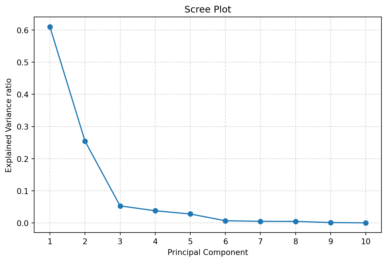
Chosen k based on turning-point elbow detection: 3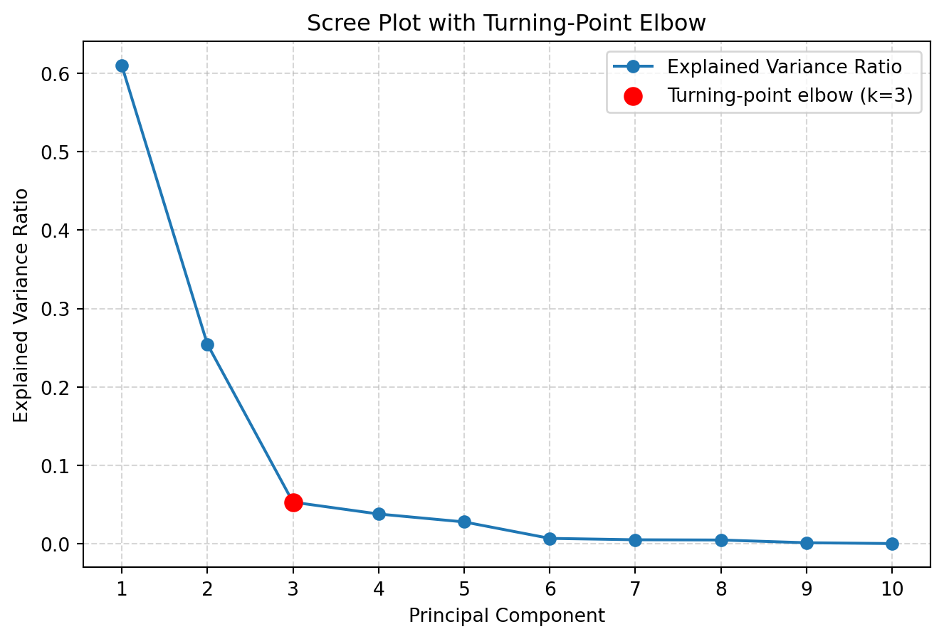
The Scree plot and Elbow method suggested using k=3 PCs for further analysis.
Task three: to validate and visualise the selected PCs
How do school look like and distribute in the top two PCs? To visualise them, we can use the following code and two PCs.
plt.figure(figsize=(7, 5))
plt.scatter(pca_np_school_reduced[:, 0],
pca_np_school_reduced[:, 1],
alpha=0.1,
edgecolor='none')
plt.xlabel(f"PC1 ({pca.explained_variance_ratio_[0]*100:.2f}% variance)")
plt.ylabel(f"PC2 ({pca.explained_variance_ratio_[1]*100:.2f}% variance)")
plt.title("PCA Scatter Plot")
plt.show()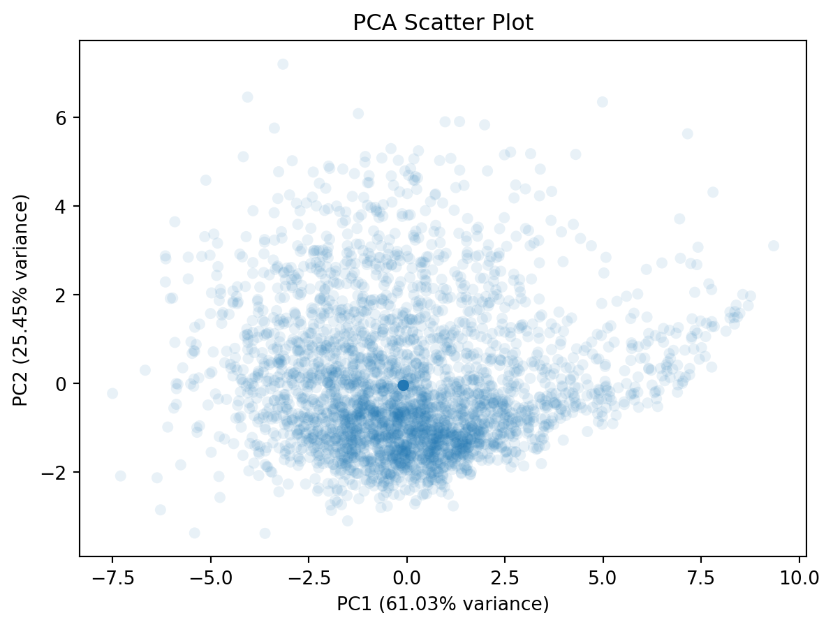
Note
If you would like to reduce the overlap between dots, you can try lowering the alpha parameter of plt.scatter(). The lower alpha, the more transparent.
This plot doesn’t tell much. We can include additional variable to this plot, such as the overall attainment 8 score for all pupils. This would reveal how the overall attainment looks like in this new feature space.
# Create DataFrame from PCA output
df_pca_school_reduced = pd.DataFrame(
    pca_np_school_reduced,
    columns=[f"PC{i}" for i in range(1, pca_np_school_reduced.shape[1]+1)] #PC1, PC2, ...
)

# Append ATT8SCR column from df_school (same row order)
df_pca_school_reduced = df_pca_school_reduced.assign(ATT8SCR = df_school.ATT8SCR)

# Plot scatter using viridis colormap
plt.figure(figsize=(7, 5))
scatter = plt.scatter(
    df_pca_school_reduced['PC1'],
    df_pca_school_reduced['PC2'],
    c=df_pca_school_reduced['ATT8SCR'],
    cmap='viridis',
    alpha=0.8,       # transparency for better visibility
    edgecolor='none'
)

# Labels and title
plt.xlabel(f"PC1 ({pca.explained_variance_ratio_[0]*100:.2f}% variance)")
plt.ylabel(f"PC2 ({pca.explained_variance_ratio_[1]*100:.2f}% variance)")
plt.title("PCA Scatter Plot Colored by ATT8SCR")

# Colorbar
plt.colorbar(scatter, label='ATT8SCR')

plt.show()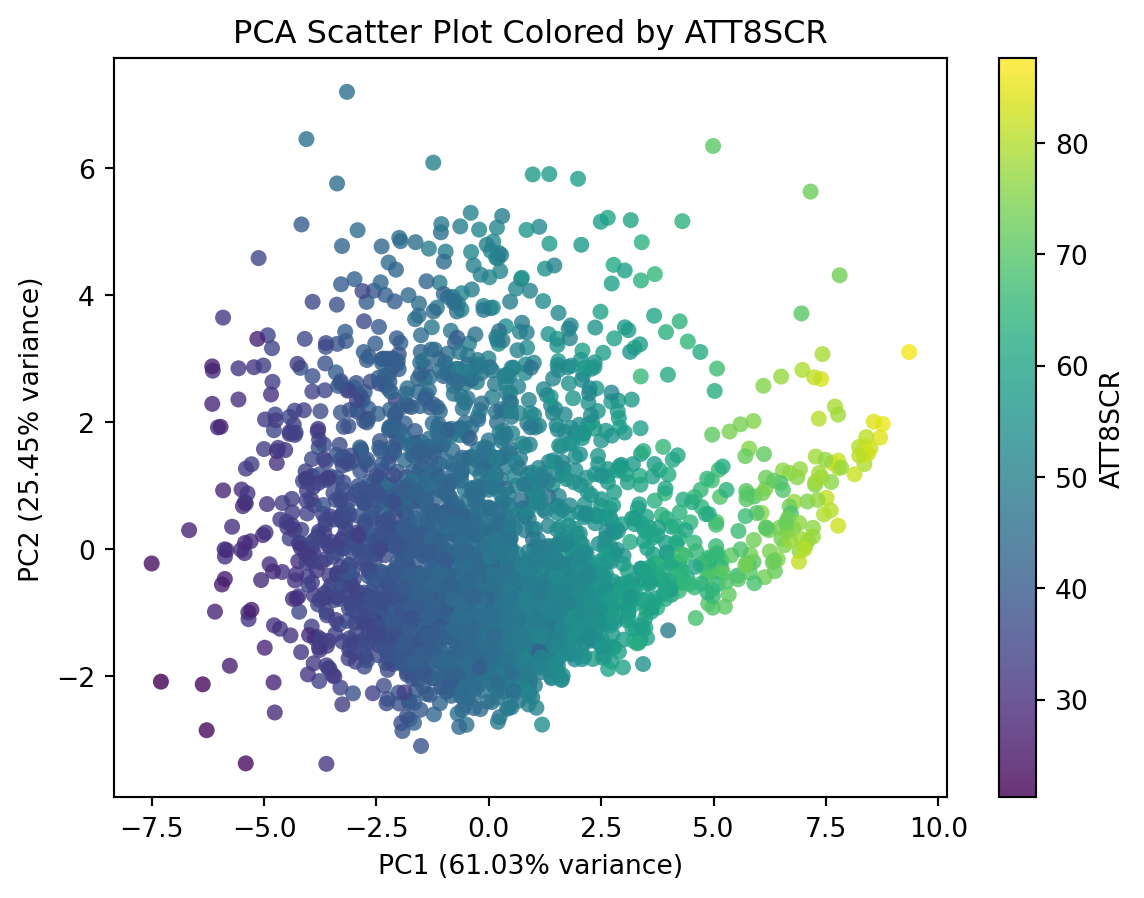
While the code above is equivalent to the code in the next cell, the code in the next cell is more concise and elegant.
# Create DataFrame from PCA output and append ATT8SCR
df_pca_school_reduced = pd.DataFrame(
    pca_np_school_reduced,
    columns=[f"PC{i}" for i in range(1, pca_np_school_reduced.shape[1] + 1)]
).assign(ATT8SCR=df_school['ATT8SCR'])

# Plot using DataFrame's plot.scatter
ax = df_pca_school_reduced.plot.scatter(
    x='PC1',
    y='PC2',
    c='ATT8SCR',
    alpha=0.8,
    figsize=(7, 5),
    edgecolor='none'
)

# Add labels and title
ax.set_xlabel(f"PC1 ({pca.explained_variance_ratio_[0]*100:.2f}% variance)")
ax.set_ylabel(f"PC2 ({pca.explained_variance_ratio_[1]*100:.2f}% variance)")
ax.set_title("PCA Scatter Plot Colored by ATT8SCR")

plt.show()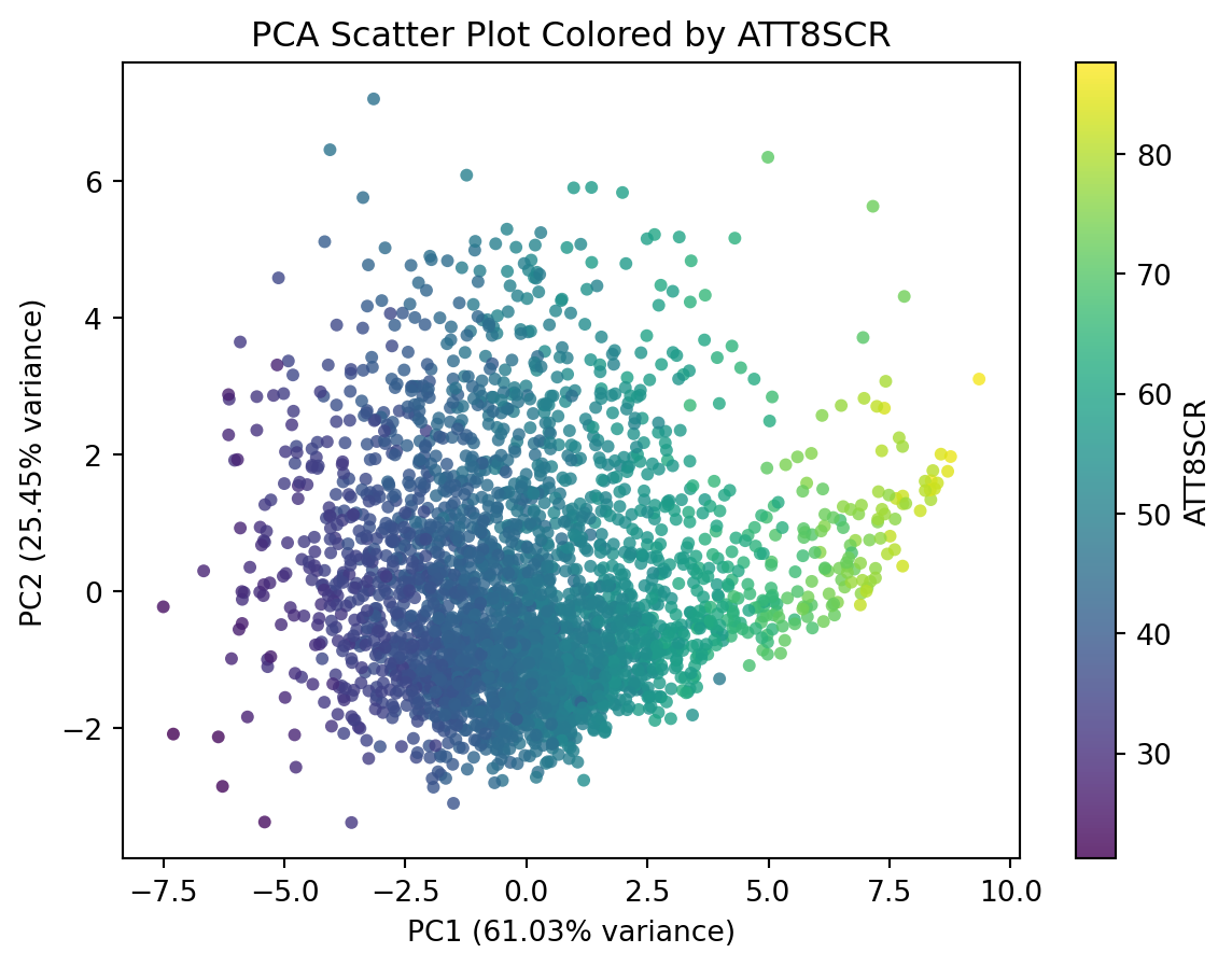
This plot shows that PC1 is higher correlated with the overall Attainment 8 score.
How about visualising absence in this new feature space?
# Append PERCTOT column from df_school
df_pca_school_reduced = ???.???(PERCTOT = df_school.???)

# Plot using DataFrame's plot.scatter
ax = df_pca_school_reduced.plot.scatter(
    x='??',
    y='??',
    c='??',
    alpha=0.8,
    figsize=(7, 5),
    edgecolor='none'
)

# Add labels and title
ax.set_xlabel(f"PC1 ({pca.explained_variance_ratio_[0]*100:.2f}% variance)")
ax.set_ylabel(f"PC2 ({pca.explained_variance_ratio_[1]*100:.2f}% variance)")
ax.set_title("PCA Scatter Plot Colored by PERCTOT")

plt.show()
df_pca_school_reduced = df_pca_school_reduced.assign(PERCTOT = df_school.PERCTOT)
# Plot using DataFrame's plot.scatter
ax = df_pca_school_reduced.plot.scatter(
x='PC1',
y='PC2',
c='PERCTOT',
alpha=0.8,
figsize=(7, 5),
edgecolor='none'
)
# Add labels and title
ax.set_xlabel(f"PC1 ({pca.explained_variance_ratio_[0]*100:.2f}% variance)")
ax.set_ylabel(f"PC2 ({pca.explained_variance_ratio_[1]*100:.2f}% variance)")
ax.set_title("PCA Scatter Plot Colored by PERCTOT")
plt.show()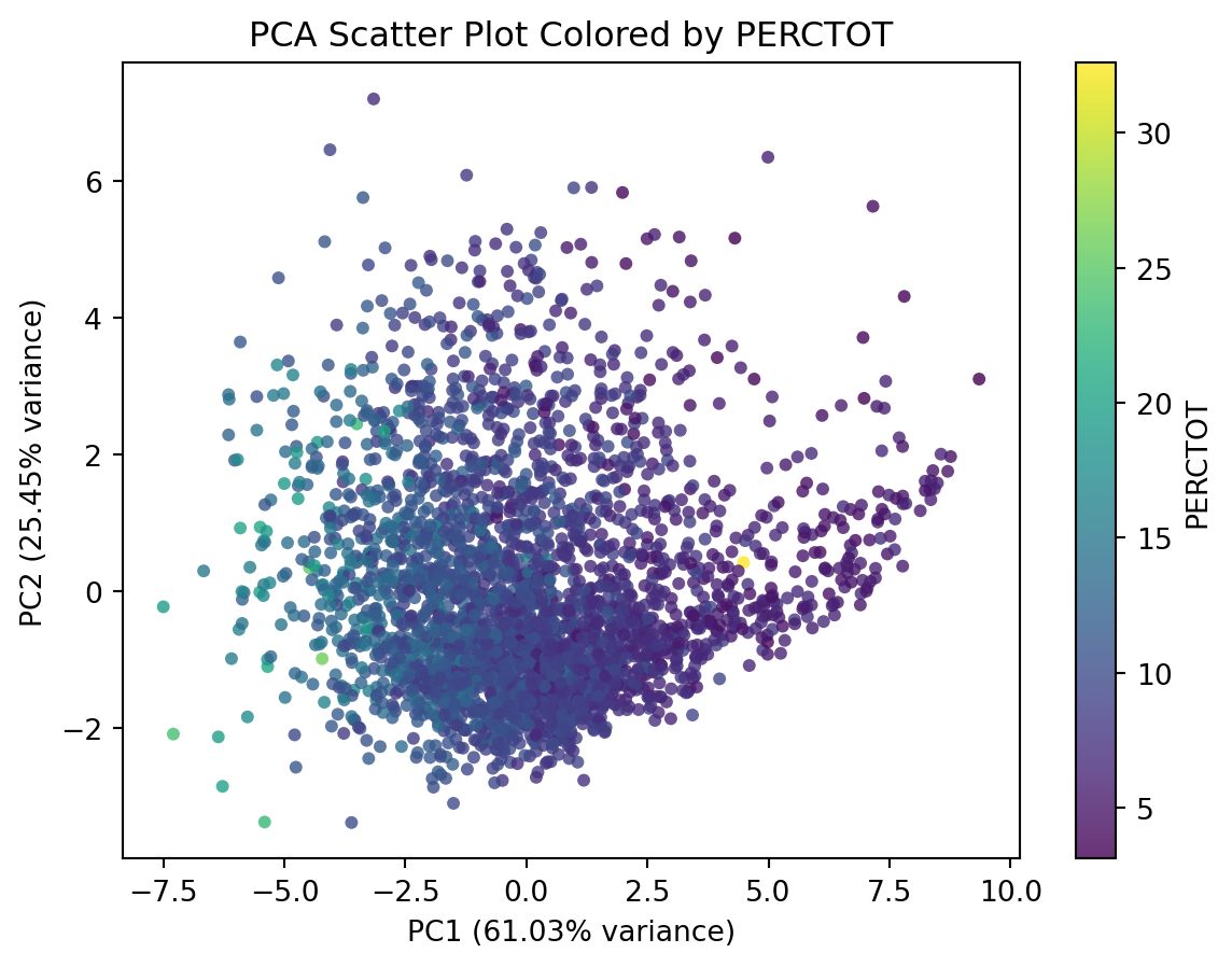
You’re Done!
Congratulations on completing the practical on dimensionality reduction.
It takes time to learn - remember practice makes perfect!
If you have time, please think about applying this technique to other variables in the school data, or your own datasets.