Dimensionality Reduction
- huanfa.chen@ucl.ac.uk
17th November 2025
CASA0007 Quantitative Methods
This week
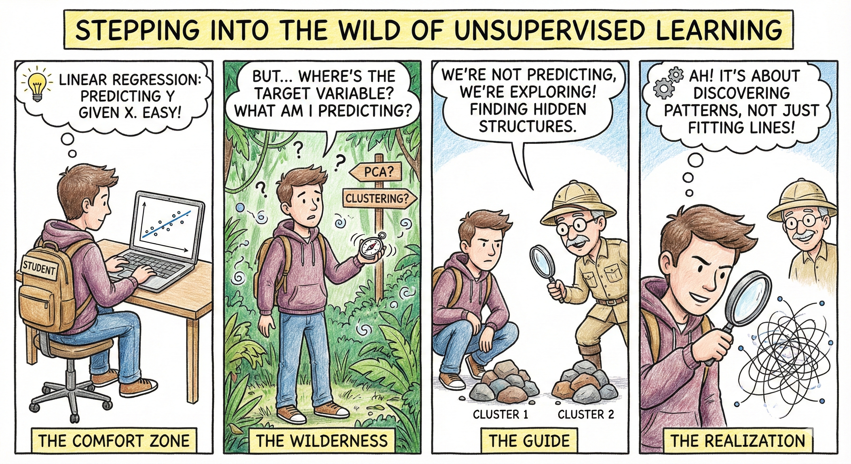
Image credit: Google GeminiDimensionality Quiz
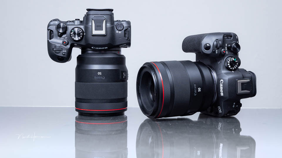
Image credit: www.photofacts.nlCanon EOR R8 has a maximum resolution of 6000 * 4000 pixels for JPEG/HEIF, where every pixel corresponds to three colour channels (RGB). What is the dimensionality of an image from EOR R8?
- A. 6000 * 4000
- B. 6000 * 4000 * 3
- C. 1
- D. 6000 * 4000 * 3 * 2
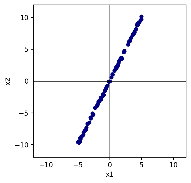
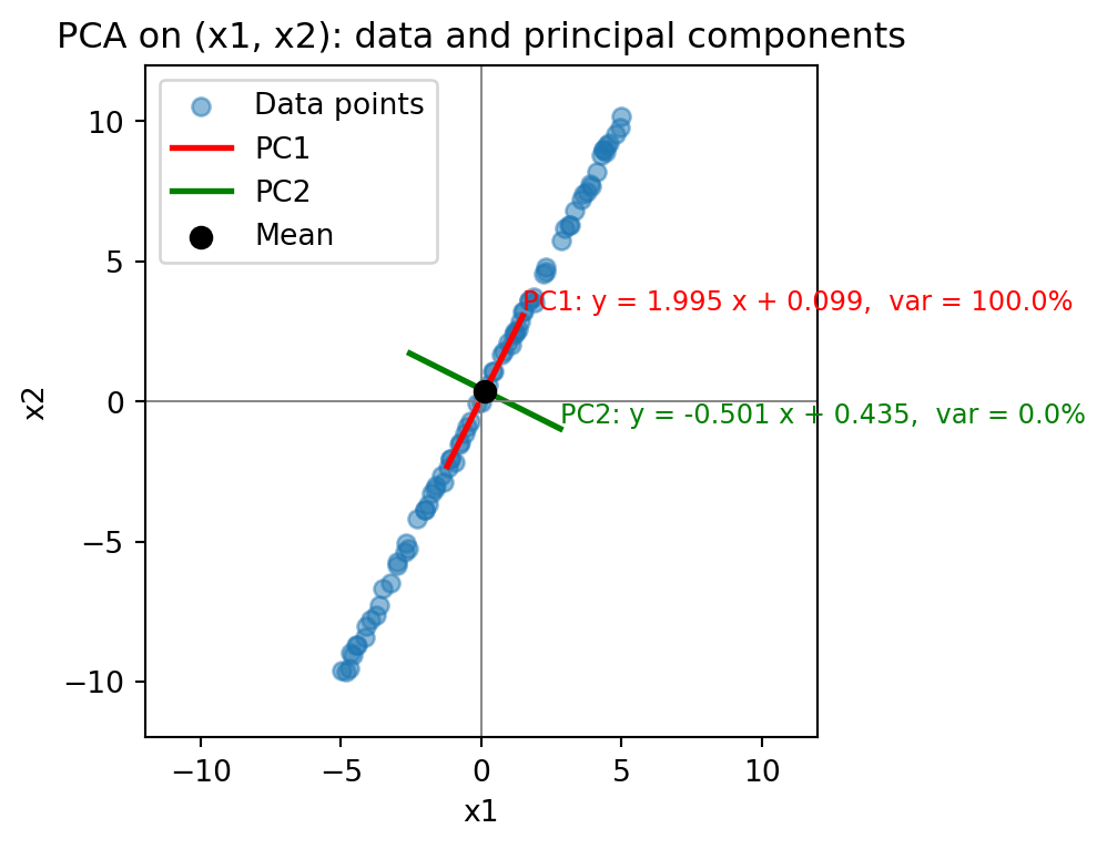
Which direction is the best?
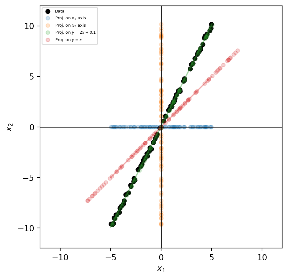
| Direction | Variance (explained) | Proportion of total |
|---|---|---|
| Original data (total) | 43.8053 | 1 |
| Projection on \(x_1\) axis | 8.79708 | 0.200822 |
| Projection on \(x_2\) axis | 35.0083 | 0.799178 |
| Projection on \(y=2x+0.1\) | 43.8013 | 0.999908 |
| Projection on \(y=x\) | 39.4468 | 0.900502 |
PCA automatically searching for informative directions
- PCA automatically searches the most informative direction, called the first principal component (PC)
- After finding this one, PCA looks for a second PC:
- Not overlapping the information already captured by the first PC
- With as spread as possible between data points
- Not needed when #1 PC explains 100% variance
Illustrating steps of PCA
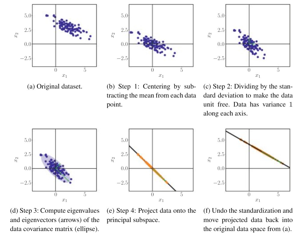
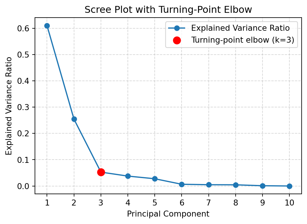
Image credit: Mathematics for Machine LearningScree plot
| n_pc | explained_var | cum_var |
|---|---|---|
| 1 | 0.61 | 0.61 |
| 2 | 0.255 | 0.865 |
| 3 | 0.053 | 0.918 |
| 4 | 0.038 | 0.955 |
| 5 | 0.028 | 0.983 |
| 6 | 0.007 | 0.99 |
| 7 | 0.005 | 0.994 |
| 8 | 0.005 | 0.999 |
| 9 | 0.001 | 1 |
| 10 | 0 | 1 |
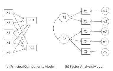
PCA is not factor analysis
- PCA aims to find PCs that are combination of original variables for maximising the variance explained.
- FA aims to find hidden factors that underlie or cause the observed variables.
Source: R in ActionExample of PCA on MNIST digit recognition
60,000 examples of handwritten digits 0~9. Each digit is an 28*28 image or 784 pixels (dimensions)
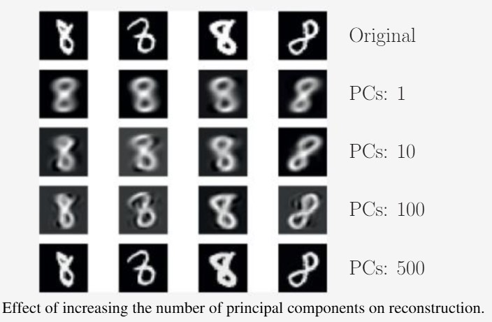
Source: Chapter 10, Mathematics for Machine Learning