Prof D’s Regression Sessions - Vol 3

AKA - In the (Linear) Mix(ed effects model practical for the next few hours)

Preamble

We’re going back in - Volume 3 of the Regression Sessions, so clearly we are going to have to have volume 4 of the Progression Sessions. Yes, “where is vol. 3?”, I hear you ask. I don’t know. Someone has lost it and it’s not up on Spotify, so we’ll have to make do and jump to volume 4 - Enjoy!

Practical Aims

Experiment with running some Linear Mixed Effects Models and converting last week’s show-stopper multiple regression model into a Linear Mixed Effects version
Practice moving from an initial null model to a fully-fledged model with fixed effects and random effects
Practice interpreting your final model and seeing if you can use it to explain which local authority-level policy might be most effective at raising attainment

Read in your data

You can use your data from last week, but I’ve created a nice clean dataset and added a few extra spicy variables about teachers and schools’ workforce in there for fun. All of that data is from here: https://explore-education-statistics.service.gov.uk/data-catalogue?themeId=b601b9ea-b1c7-4970-b354-d1f695c446f1&sortBy=newest&geographicLevel=SCH

To save time, you might just want to download it directly from here: https://github.com/adamdennett/QM/blob/main/sessions/L6_data/Performancetables_130242/2022-2023/school_data_2223.csv

Code


import pandas as pd
import numpy as np
import janitor
from pathlib import Path
import statsmodels.api as sm

# little function to define the file root on different machines
def find_qm_root(start_path: Path = Path.cwd(), anchor: str = "QM") -> Path:
    """
    Traverse up from the start_path until the anchor folder (e.g. 'QM' or 'QM_Fork')      is found. Returns the path to the anchor folder.
    """
    for parent in [start_path] + list(start_path.parents):
        if parent.name == anchor:
            return parent
    raise FileNotFoundError(f"Anchor folder '{anchor}' not found in path      hierarchy.")
  
qm_root = find_qm_root()
base_path = qm_root / "sessions" / "L6_data" / "Performancetables_130242" / "2022-2023"
na_all = ["", "NA", "SUPP", "NP", "NE", "SP", "SN", "LOWCOV", "NEW", "SUPPMAT", "NaN"]

qm_root = find_qm_root()
base_path = qm_root / "sessions" / "L6_data" / "Performancetables_130242" / "2022-2023"
na_all = ["", "NA", "SUPP", "NP", "NE", "SP", "SN", "LOWCOV", "NEW", "SUPPMAT", "NaN"]

england_filtered = pd.read_csv(base_path / "school_data_2223.csv", na_values=na_all, dtype={"URN": str})

# Log-transform safely: replace non-positive values with NaN
england_filtered['log_ATT8SCR'] = np.where(england_filtered['ATT8SCR'] > 0, np.log(england_filtered['ATT8SCR']), np.nan)
england_filtered['log_PTFSM6CLA1A'] = np.where(england_filtered['PTFSM6CLA1A'] > 0, np.log(england_filtered['PTFSM6CLA1A']), np.nan)

# Drop rows with NaNs in either column
england_filtered_clean = england_filtered.dropna(subset=['log_ATT8SCR', 'log_PTFSM6CLA1A'])

Code

library(tidyverse)

## Note edit your base path to refer to the folder where you have stored your data
base_path <- here("sessions", "L6_data", "Performancetables_130242", "2022-2023")
na_all <- c("", "NA", "SUPP", "NP", "NE", "SP", "SN", "LOWCOV", "NEW", "SUPPMAT")

england_filtered <- read_csv(file.path(base_path, "school_data_2223.csv"), na = na_all) |> mutate(URN = as.character(URN))

#str(england_filtered)

england_filtered_clean <- england_filtered[
  !is.na(england_filtered$ATT8SCR) & 
  !is.na(england_filtered$PTFSM6CLA1A) &
  england_filtered$ATT8SCR > 0 &
  england_filtered$PTFSM6CLA1A > 0, 
]

The Warm-up - Last week’s Multiple Regression Show Stopper

To get us going we are going to run our ‘show-stopper’ model from last week so that we can compare this with a final linear mixed effects version at the end of the practical.
You should run your best model (without any interaction effects) from last week, however, to help you along my best model from last week looked like this:

Code

import numpy as np
import statsmodels.formula.api as smf

# Filter rows where all log-transformed variables are > 0
england_filtered_clean = england_filtered_clean[
    (england_filtered_clean['PTFSM6CLA1A'] > 0) &
    (england_filtered_clean['PERCTOT'] > 0) &
    (england_filtered_clean['PNUMEAL'] > 0)
].copy()

# Create log-transformed columns
england_filtered_clean['log_ATT8SCR'] = np.log(england_filtered_clean['ATT8SCR'])
england_filtered_clean['log_PTFSM6CLA1A'] = np.log(england_filtered_clean['PTFSM6CLA1A'])
england_filtered_clean['log_PERCTOT'] = np.log(england_filtered_clean['PERCTOT'])
england_filtered_clean['log_PNUMEAL'] = np.log(england_filtered_clean['PNUMEAL'])

# Fit the model
model = smf.ols(
    formula='log_ATT8SCR ~ log_PTFSM6CLA1A + log_PERCTOT + log_PNUMEAL + OFSTEDRATING + gor_name + PTPRIORLO + ADMPOL_PT',
    data=england_filtered_clean
).fit()

print(model.summary())

                            OLS Regression Results                            
==============================================================================
Dep. Variable:            log_ATT8SCR   R-squared:                       0.844
Model:                            OLS   Adj. R-squared:                  0.843
Method:                 Least Squares   F-statistic:                     868.5
Date:                Tue, 09 Dec 2025   Prob (F-statistic):               0.00
Time:                        21:04:57   Log-Likelihood:                 3411.9
No. Observations:                2902   AIC:                            -6786.
Df Residuals:                    2883   BIC:                            -6672.
Df Model:                          18                                         
Covariance Type:            nonrobust                                         
========================================================================================================
                                           coef    std err          t      P>|t|      [0.025      0.975]
--------------------------------------------------------------------------------------------------------
Intercept                                4.6270      0.016    280.473      0.000       4.595       4.659
OFSTEDRATING[T.Outstanding]              0.0552      0.004     12.597      0.000       0.047       0.064
OFSTEDRATING[T.Requires improvement]    -0.0517      0.005    -11.427      0.000      -0.061      -0.043
OFSTEDRATING[T.Serious Weaknesses]      -0.0603      0.016     -3.715      0.000      -0.092      -0.028
OFSTEDRATING[T.Special Measures]        -0.0952      0.019     -5.017      0.000      -0.132      -0.058
gor_name[T.East of England]              0.0057      0.006      0.897      0.370      -0.007       0.018
gor_name[T.London]                       0.0267      0.007      4.078      0.000       0.014       0.040
gor_name[T.North East]                   0.0203      0.008      2.405      0.016       0.004       0.037
gor_name[T.North West]                  -0.0139      0.006     -2.287      0.022      -0.026      -0.002
gor_name[T.South East]                  -0.0128      0.006     -2.119      0.034      -0.025      -0.001
gor_name[T.South West]                   0.0254      0.007      3.863      0.000       0.013       0.038
gor_name[T.West Midlands]                0.0059      0.006      0.931      0.352      -0.006       0.018
gor_name[T.Yorkshire and the Humber]     0.0200      0.007      3.046      0.002       0.007       0.033
ADMPOL_PT[T.OTHER NON SEL]               0.0154      0.006      2.529      0.011       0.003       0.027
ADMPOL_PT[T.SEL]                         0.0807      0.010      8.210      0.000       0.061       0.100
log_PTFSM6CLA1A                         -0.0699      0.004    -18.950      0.000      -0.077      -0.063
log_PERCTOT                             -0.2245      0.007    -30.152      0.000      -0.239      -0.210
log_PNUMEAL                              0.0180      0.002     11.109      0.000       0.015       0.021
PTPRIORLO                               -0.0069      0.000    -31.525      0.000      -0.007      -0.007
==============================================================================
Omnibus:                      117.971   Durbin-Watson:                   1.799
Prob(Omnibus):                  0.000   Jarque-Bera (JB):              180.406
Skew:                          -0.370   Prob(JB):                     6.69e-40
Kurtosis:                       3.972   Cond. No.                         346.
==============================================================================

Notes:
[1] Standard Errors assume that the covariance matrix of the errors is correctly specified.

Code

england_filtered_clean <- england_filtered_clean %>%
  filter(PTFSM6CLA1A > 0, PERCTOT > 0, PNUMEAL > 0)

england_model7 <- lm(log(ATT8SCR) ~ log(PTFSM6CLA1A) + log(PERCTOT) + log(PNUMEAL) + OFSTEDRATING + gor_name + PTPRIORLO + ADMPOL_PT, data = england_filtered_clean, na.action = na.exclude)
summary(england_model7)


Call:
lm(formula = log(ATT8SCR) ~ log(PTFSM6CLA1A) + log(PERCTOT) + 
    log(PNUMEAL) + OFSTEDRATING + gor_name + PTPRIORLO + ADMPOL_PT, 
    data = england_filtered_clean, na.action = na.exclude)

Residuals:
     Min       1Q   Median       3Q      Max 
-0.37723 -0.04528  0.00333  0.04912  0.30081 

Coefficients:
                                   Estimate Std. Error t value Pr(>|t|)    
(Intercept)                       4.6270385  0.0164972 280.473  < 2e-16 ***
log(PTFSM6CLA1A)                 -0.0699264  0.0036900 -18.950  < 2e-16 ***
log(PERCTOT)                     -0.2244960  0.0074455 -30.152  < 2e-16 ***
log(PNUMEAL)                      0.0179676  0.0016174  11.109  < 2e-16 ***
OFSTEDRATINGOutstanding           0.0551690  0.0043794  12.597  < 2e-16 ***
OFSTEDRATINGRequires improvement -0.0516629  0.0045211 -11.427  < 2e-16 ***
OFSTEDRATINGSerious Weaknesses   -0.0602663  0.0162207  -3.715 0.000207 ***
OFSTEDRATINGSpecial Measures     -0.0951661  0.0189679  -5.017 5.56e-07 ***
gor_nameEast of England           0.0056999  0.0063522   0.897 0.369630    
gor_nameLondon                    0.0266978  0.0065474   4.078 4.67e-05 ***
gor_nameNorth East                0.0202813  0.0084342   2.405 0.016250 *  
gor_nameNorth West               -0.0139159  0.0060835  -2.287 0.022239 *  
gor_nameSouth East               -0.0128394  0.0060587  -2.119 0.034161 *  
gor_nameSouth West                0.0254495  0.0065872   3.863 0.000114 ***
gor_nameWest Midlands             0.0058630  0.0063008   0.931 0.352183    
gor_nameYorkshire and the Humber  0.0199996  0.0065661   3.046 0.002341 ** 
PTPRIORLO                        -0.0069371  0.0002201 -31.525  < 2e-16 ***
ADMPOL_PTOTHER NON SEL            0.0154098  0.0060930   2.529 0.011488 *  
ADMPOL_PTSEL                      0.0806871  0.0098281   8.210 3.30e-16 ***
---
Signif. codes:  0 '***' 0.001 '**' 0.01 '*' 0.05 '.' 0.1 ' ' 1

Residual standard error: 0.07492 on 2883 degrees of freedom
  (59 observations deleted due to missingness)
Multiple R-squared:  0.8443,    Adjusted R-squared:  0.8433 
F-statistic: 868.5 on 18 and 2883 DF,  p-value: < 2.2e-16

Building Our Linear Mixed Effects Model

Stage 1 - The Null / Variance Components Model for Ofsted Ratings

If you remember from the lecture, in order to determine whether running a linear mixed effects / multilevel model is necessary, if you have categorical / grouping factors in your data set (random effects), you should run the null model to see how much variance the groups in your data are explaining.
In our data, we had a couple of different grouping variable candidates:
- Ofsted Rating (how ‘good’ or otherwise a school is as determined by the Office for Standards in Education - Ofsted)
- Geographical groups. In our data these are Regions and the Local Authorities within those regions.
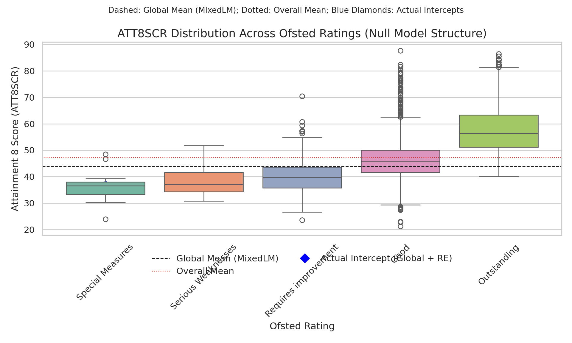
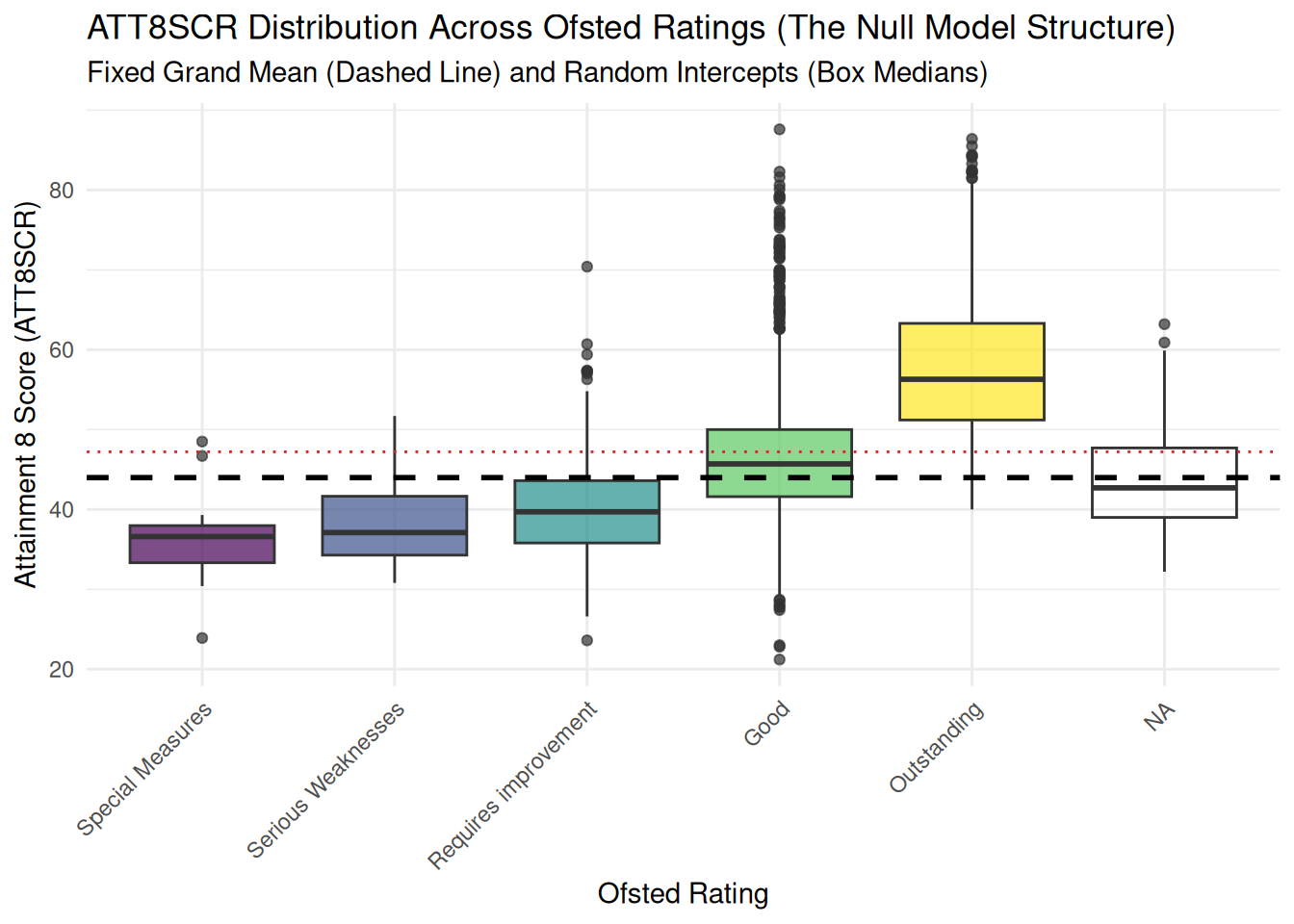
Below is some code to visualise those groups as boxplots.

Code

import pandas as pd
import numpy as np
import statsmodels.api as sm
import seaborn as sns
import matplotlib.pyplot as plt
from matplotlib.lines import Line2D

sns.set_theme(style="whitegrid")

# --- Ensure OFSTEDRATING is clean and categorical ---
rating_order = ["Special Measures", "Serious Weaknesses", "Requires improvement", "Good", "Outstanding"]
england_filtered_clean["OFSTEDRATING"] = england_filtered_clean["OFSTEDRATING"].astype(str)
england_filtered_clean["OFSTEDRATING"] = pd.Categorical(
    england_filtered_clean["OFSTEDRATING"],
    categories=rating_order,
    ordered=True
)

# --- Keep valid rows (ATT8SCR present and rating in our order) ---
df = england_filtered_clean.dropna(subset=["ATT8SCR"]).copy()
df = df[df["OFSTEDRATING"].isin(rating_order)]

# --- Fit MixedLM null model (random intercept by OFSTEDRATING) ---
mixed_model = sm.MixedLM.from_formula("ATT8SCR ~ 1", groups="OFSTEDRATING", data=df)
mixed_fit = mixed_model.fit(method="lbfgs")

# --- Global mean (fixed intercept) ---
global_mean = mixed_fit.params["Intercept"] if "Intercept" in mixed_fit.params.index else float(mixed_fit.params.iloc[0])

# --- Robust random-effects extraction ---
def get_re_value(effect):
    # effect may be a pandas Series (with/without 'Intercept'), ndarray, or list
    if isinstance(effect, pd.Series):
        return float(effect["Intercept"]) if "Intercept" in effect.index else float(effect.iloc[0])
    arr = np.asarray(effect).ravel()
    return float(arr[0]) if arr.size > 0 else np.nan

random_effects = mixed_fit.random_effects  # dict: {group_label: effect_vector}
group_effects = {str(k): get_re_value(v) for k, v in random_effects.items()}

ranef_df = pd.DataFrame({
    "OFSTEDRATING": list(group_effects.keys()),
    "ranef": list(group_effects.values())
}).sort_values("OFSTEDRATING")

# --- Actual intercepts = global mean + random effect ---
ranef_df["actual_intercept"] = global_mean + ranef_df["ranef"]

# --- Overall mean from raw data ---
overall_mean = df["ATT8SCR"].mean()

# --- Plot: boxplots + lines + actual intercept markers ---
fig, ax = plt.subplots(figsize=(10, 6))
sns.boxplot(data=df, x="OFSTEDRATING", y="ATT8SCR", palette="Set2", ax=ax)

# Reference lines
ax.axhline(global_mean, color="black", linestyle="--", linewidth=1)
ax.axhline(overall_mean, color="#d62728", linestyle=":", linewidth=1)

# Overlay actual intercepts (blue diamonds) per rating
sns.scatterplot(
    data=ranef_df,
    x="OFSTEDRATING", y="actual_intercept",
    marker="D", s=100, color="blue",
    ax=ax
)

# Titles & labels
ax.set_title("ATT8SCR Distribution Across Ofsted Ratings (Null Model Structure)", fontsize=14)
fig.suptitle("Dashed: Global Mean (MixedLM); Dotted: Overall Mean; Blue Diamonds: Actual Intercepts", fontsize=10)
ax.set_xlabel("Ofsted Rating")
ax.set_ylabel("Attainment 8 Score (ATT8SCR)")
plt.xticks(rotation=45)

([0, 1, 2, 3, 4], [Text(0, 0, 'Special Measures'), Text(1, 0, 'Serious Weaknesses'), Text(2, 0, 'Requires improvement'), Text(3, 0, 'Good'), Text(4, 0, 'Outstanding')])

Code

# --- Manual legend handles (prevents 'Axes has no legend attached') ---
legend_handles = [
    Line2D([0], [0], color='black', linestyle='--', linewidth=1, label='Global Mean (MixedLM)'),
    Line2D([0], [0], color='#d62728', linestyle=':', linewidth=1, label='Overall Mean'),
    Line2D([0], [0], marker='D', color='blue', linestyle='None', markersize=8, label='Actual Intercept (Global + RE)')
]
ax.legend(legend_handles, [h.get_label() for h in legend_handles],
          loc="lower center", bbox_to_anchor=(0.5, -0.25), ncol=2, frameon=False)

plt.tight_layout()
plt.show()

Code

# 1. Load the necessary library for plotting
library(ggplot2)
library(lme4)

# --- Ensure OFSTEDRATING is an ordered factor for better plotting ---
# It appears you have six levels based on the OLS output, so we order them logically.
# Adjust the order if the true levels/baseline are different in your data.
rating_order <- c("Special Measures", "Serious Weaknesses", "Requires improvement", "Good", "Outstanding")
england_filtered_clean$OFSTEDRATING <- factor(
  england_filtered_clean$OFSTEDRATING,
  levels = rating_order,
  ordered = TRUE
)

#Fit the model
lme1 <- lmer(ATT8SCR ~ 1 + (1 | OFSTEDRATING), data = england_filtered_clean)
# Extract the fixed-effect intercept and store in a variable
global_mean <- fixef(lme1)[1]
# Check the value
global_mean

(Intercept) 
   43.98243

Code

## ## 1. Boxplot Visualization (Level 1 and Level 2 Variance) ## ##
boxplot_att8scr <- ggplot(england_filtered_clean, aes(x = OFSTEDRATING, y = ATT8SCR, fill = OFSTEDRATING)) +
  geom_boxplot(alpha = 0.7) +
  geom_hline(yintercept = global_mean, linetype = "dashed", color = "black", linewidth = 1) +
  geom_hline(yintercept = mean(england_filtered_clean$ATT8SCR, na.rm = TRUE), linetype = "dotted", color = "#d62728", linewidth = 0.5) +
  labs(title = "ATT8SCR Distribution Across Ofsted Ratings (The Null Model Structure)",
       subtitle = "Fixed Grand Mean (Dashed Line) and Random Intercepts (Box Medians)",
       x = "Ofsted Rating",
       y = "Attainment 8 Score (ATT8SCR)") +
  theme_minimal() +
  theme(axis.text.x = element_text(angle = 45, hjust = 1), legend.position = "none")

print(boxplot_att8scr)

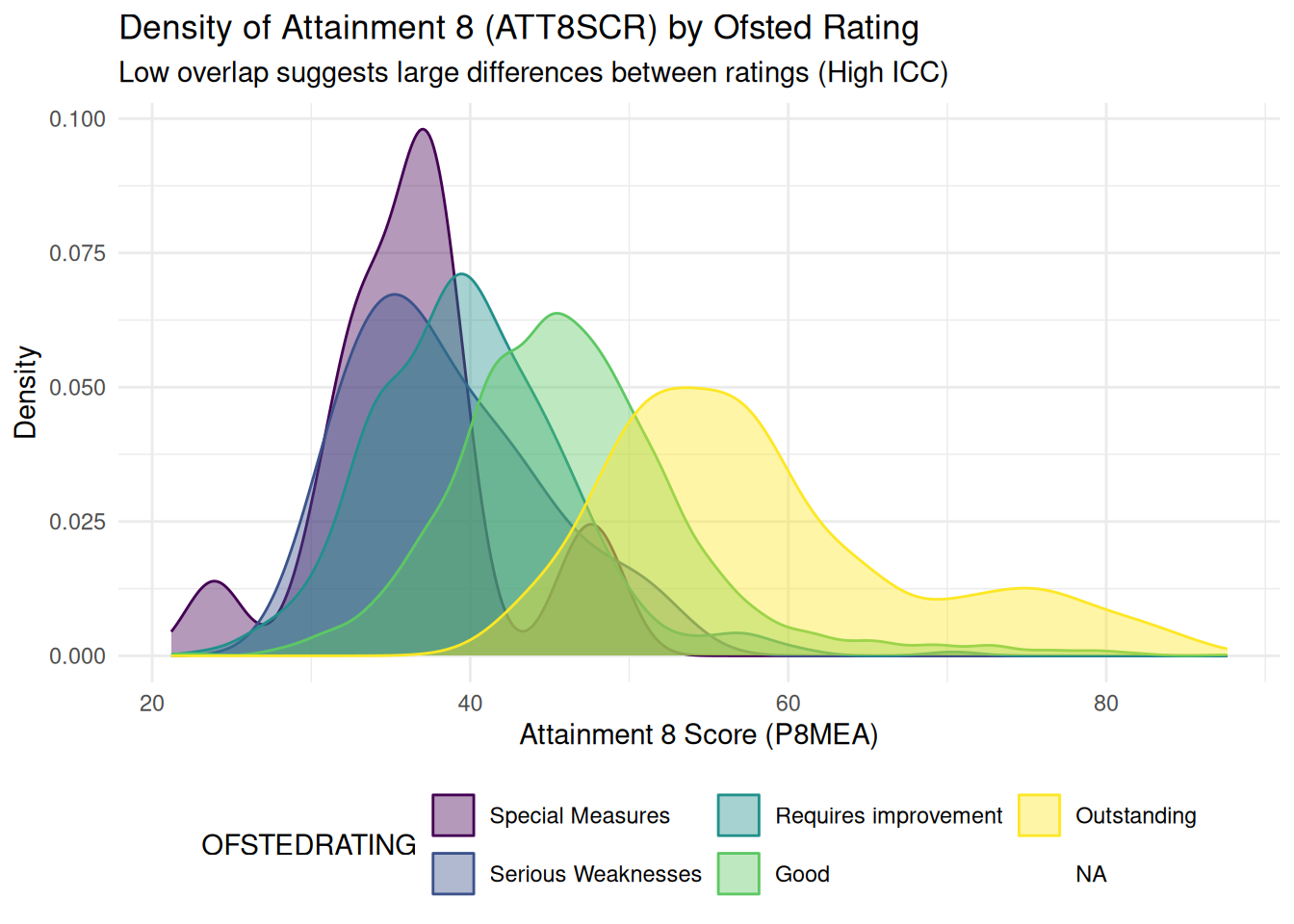
The Interclass Correlation Coefficient - ICC

Again, if you recall from the lecture, the ICC is simply the ratio between the between the between group variance and the total variance
The higher the ICC (closer to 1), the more variance is due to differences between groups (i.e. differences between the Ofsted rating of schools) than within groups (i.e. between schools within Ofsted rating bands)
This can be judged visually with a stacked density plot:
- High ICC = distinct, non-overlapping humps
- Low ICC = density plots all overlapping on-top of each other
Remember A high ICC is a strong indication that a multilevel / mixed effects model is a suitable modelling strategy to pursue to try and explain these group-level differences

Code

import pandas as pd
import seaborn as sns
import matplotlib.pyplot as plt

sns.set_theme(style="whitegrid")

rating_order = ["Special Measures", "Serious Weaknesses", "Requires improvement", "Good", "Outstanding"]
england_filtered_clean["OFSTEDRATING"] = pd.Categorical(
    england_filtered_clean["OFSTEDRATING"],
    categories=rating_order,
    ordered=True
)

plot_df = england_filtered_clean.dropna(subset=["ATT8SCR", "OFSTEDRATING"]).copy()

# Create figure and axis manually
fig, ax = plt.subplots(figsize=(8, 5))

# Plot KDE for each category
for rating in rating_order:
    subset = plot_df[plot_df["OFSTEDRATING"] == rating]
    sns.kdeplot(
        data=subset,
        x="ATT8SCR",
        fill=True,
        alpha=0.4,
        linewidth=1.2,
        ax=ax,
        label=rating
    )

# Titles & labels
ax.set_title("Density of Attainment 8 (ATT8SCR) by Ofsted Rating", fontsize=14)
ax.set_xlabel("Attainment 8 Score (ATT8SCR)")
ax.set_ylabel("Density")
ax.legend(title="Ofsted Rating", loc="lower center", bbox_to_anchor=(0.5, -0.25), ncol=3)

plt.tight_layout()
plt.show()

Code

## ## 2. Density Plot Visualization (Comparing the Two Variance Components) ## ##
# This plot visually shows how much the groups overlap (small overlap means high ICC).
density_att8scr <- ggplot(england_filtered_clean, aes(x = ATT8SCR, fill = OFSTEDRATING, color = OFSTEDRATING)) +
  geom_density(alpha = 0.4) +
  labs(
    title = "Density of Attainment 8 (ATT8SCR) by Ofsted Rating",
    subtitle = "Low overlap suggests large differences between ratings (High ICC)",
    x = "Attainment 8 Score (P8MEA)",
    y = "Density"
  ) +
  theme_minimal() +
  theme(legend.position = "bottom")

print(density_att8scr)

Running the Null Model and Calculating the Inter-Class Correlation Coefficient (ICC)

You will also remember from the lecture, that we can run our null model using standard statistical software. - In R, we use the lmer package, whereas in Python for now we’ll use statsmodels
First run the model as below:

Code

import pandas as pd
import statsmodels.api as sm

# Ensure OFSTEDRATING is categorical
rating_order = ["Special Measures", "Serious Weaknesses", "Requires improvement", "Good", "Outstanding"]
england_filtered_clean["OFSTEDRATING"] = pd.Categorical(
    england_filtered_clean["OFSTEDRATING"],
    categories=rating_order,
    ordered=True
)

# Drop missing values for P8MEA and OFSTEDRATING
df = england_filtered_clean.dropna(subset=["ATT8SCR", "OFSTEDRATING"]).copy()

# Fit null model: random intercept for OFSTEDRATING
null_model = sm.MixedLM.from_formula("ATT8SCR ~ 1", groups="OFSTEDRATING", data=df)
null_fit = null_model.fit()

# Summary
print(null_fit.summary())

           Mixed Linear Model Regression Results
===========================================================
Model:              MixedLM Dependent Variable: ATT8SCR    
No. Observations:   2902    Method:             REML       
No. Groups:         5       Scale:              60.9126    
Min. group size:    16      Log-Likelihood:     -10091.1281
Max. group size:    2076    Converged:          Yes        
Mean group size:    580.4                                  
-----------------------------------------------------------
                 Coef.  Std.Err.   z    P>|z| [0.025 0.975]
-----------------------------------------------------------
Intercept        43.982    3.976 11.063 0.000 36.190 51.775
OFSTEDRATING Var 77.648    7.129                           
===========================================================

Code

library(lme4)
library(performance)

#lm1 <- lm(P8MEA ~ PTFSM6CLA1A + OFSTEDRATING, data = england_filtered_clean)
#summary(lm1)

lme1 <- lmer(ATT8SCR ~ 1 + (1|OFSTEDRATING), data = england_filtered_clean)
summary(lme1)

Linear mixed model fit by REML ['lmerMod']
Formula: ATT8SCR ~ 1 + (1 | OFSTEDRATING)
   Data: england_filtered_clean

REML criterion at convergence: 20182.3

Scaled residuals: 
    Min      1Q  Median      3Q     Max 
-3.2237 -0.6418 -0.1102  0.4778  5.2840 

Random effects:
 Groups       Name        Variance Std.Dev.
 OFSTEDRATING (Intercept) 77.68    8.814   
 Residual                 60.91    7.805   
Number of obs: 2902, groups:  OFSTEDRATING, 5

Fixed effects:
            Estimate Std. Error t value
(Intercept)   43.982      3.976   11.06

Once we have run the model we can calculate the ICC:

Code

var_components = null_fit.cov_re.iloc[0, 0]  # random intercept variance
resid_var = null_fit.scale                   # residual variance
icc = var_components / (var_components + resid_var)
print(f"ICC: {icc:.3f}")

ICC: 0.560

Code

library(performance)

icc_value <- performance::icc(lme1, by_group = T)
print(icc_value)

# ICC by Group

Group        |   ICC
--------------------
OFSTEDRATING | 0.560

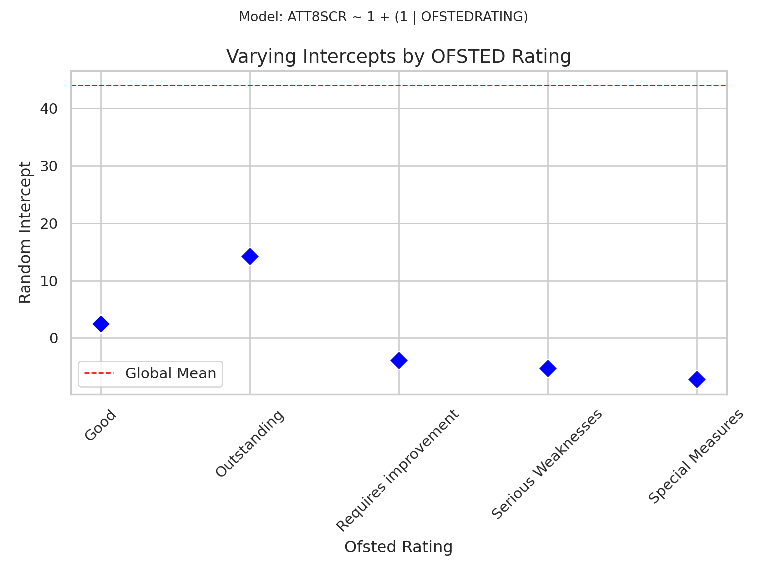
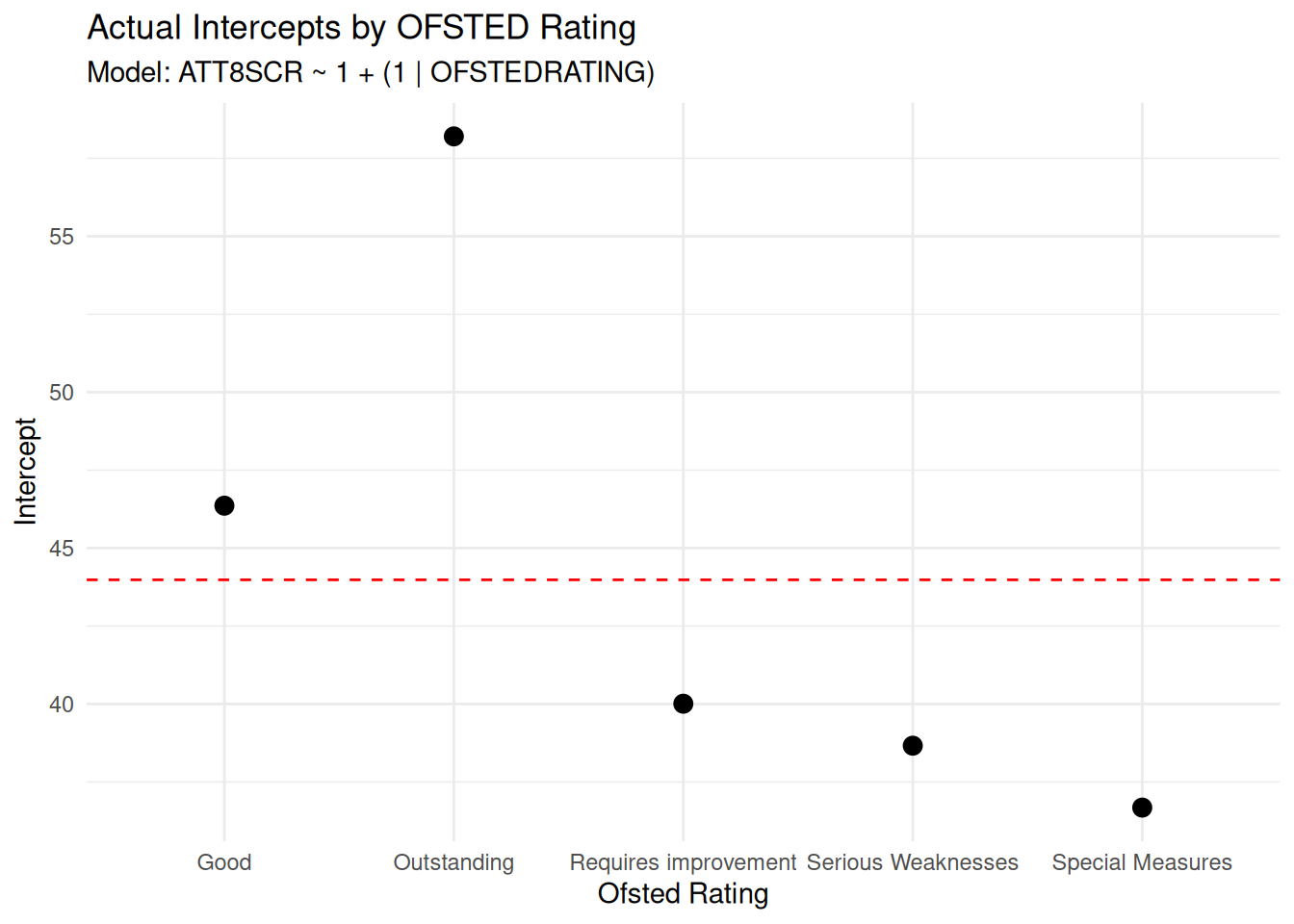
Null Model Visualisation

You will know by know that I am a big advovate of visualising everything as we go, so here is a visualisation of the null model which shows the different intercept values for the different group
Remember, we can think of the intercept as the ‘baseline’ expected for our dependent variable

Code

import pandas as pd
import statsmodels.api as sm
import seaborn as sns
import matplotlib.pyplot as plt

# Ensure OFSTEDRATING is categorical
rating_order = ["Special Measures", "Serious Weaknesses", "Requires improvement", "Good", "Outstanding"]
england_filtered_clean["OFSTEDRATING"] = pd.Categorical(
    england_filtered_clean["OFSTEDRATING"],
    categories=rating_order,
    ordered=True
)

# Drop missing values
df = england_filtered_clean.dropna(subset=["ATT8SCR", "OFSTEDRATING"]).copy()

# Fit null model: random intercept for OFSTEDRATING
null_model = sm.MixedLM.from_formula("ATT8SCR ~ 1", groups="OFSTEDRATING", data=df)
null_fit = null_model.fit()

# Extract global mean (fixed effect intercept)
global_mean = null_fit.params["Intercept"]

# Extract random effects for each group (take first value from each Series)
random_effects = null_fit.random_effects
ranef_df = pd.DataFrame({
    "OFSTEDRATING": list(random_effects.keys()),
    "Intercept": [float(effect.iloc[0]) for effect in random_effects.values()]
})

# Plot random intercepts
plt.figure(figsize=(8, 6))
sns.scatterplot(data=ranef_df, x="OFSTEDRATING", y="Intercept", s=100, color="blue", marker="D")

# Add dashed line for global mean
plt.axhline(global_mean, color="red", linestyle="--", linewidth=1, label="Global Mean")

# Titles and labels
plt.title("Varying Intercepts by OFSTED Rating", fontsize=14)
plt.suptitle("Model: ATT8SCR ~ 1 + (1 | OFSTEDRATING)", fontsize=10)
plt.xlabel("Ofsted Rating")
plt.ylabel("Random Intercept")
plt.xticks(rotation=45)

([0, 1, 2, 3, 4], [Text(0, 0, 'Good'), Text(1, 0, 'Outstanding'), Text(2, 0, 'Requires improvement'), Text(3, 0, 'Serious Weaknesses'), Text(4, 0, 'Special Measures')])

Code

plt.legend()
plt.tight_layout()
plt.show()

Code

library(lme4)
library(ggplot2)

# Fit the model
lme1 <- lmer(ATT8SCR ~ 1 + (1|OFSTEDRATING), data = england_filtered_clean)

# Extract random effects
ranef_df <- as.data.frame(ranef(lme1)$OFSTEDRATING)
ranef_df$OFSTEDRATING <- rownames(ranef(lme1)$OFSTEDRATING)

ranef_df$actual_intercept <- ranef_df$`(Intercept)` + fixef(lme1)[1]

ggplot(ranef_df, aes(x = OFSTEDRATING, y = actual_intercept)) +
  geom_point(size = 3) +
  geom_hline(yintercept = fixef(lme1)[1], linetype = "dashed", color = "red") +
  labs(title = "Actual Intercepts by OFSTED Rating",
       subtitle = "Model: ATT8SCR ~ 1 + (1 | OFSTEDRATING)",
       x = "Ofsted Rating",
       y = "Intercept") +
  theme_minimal()

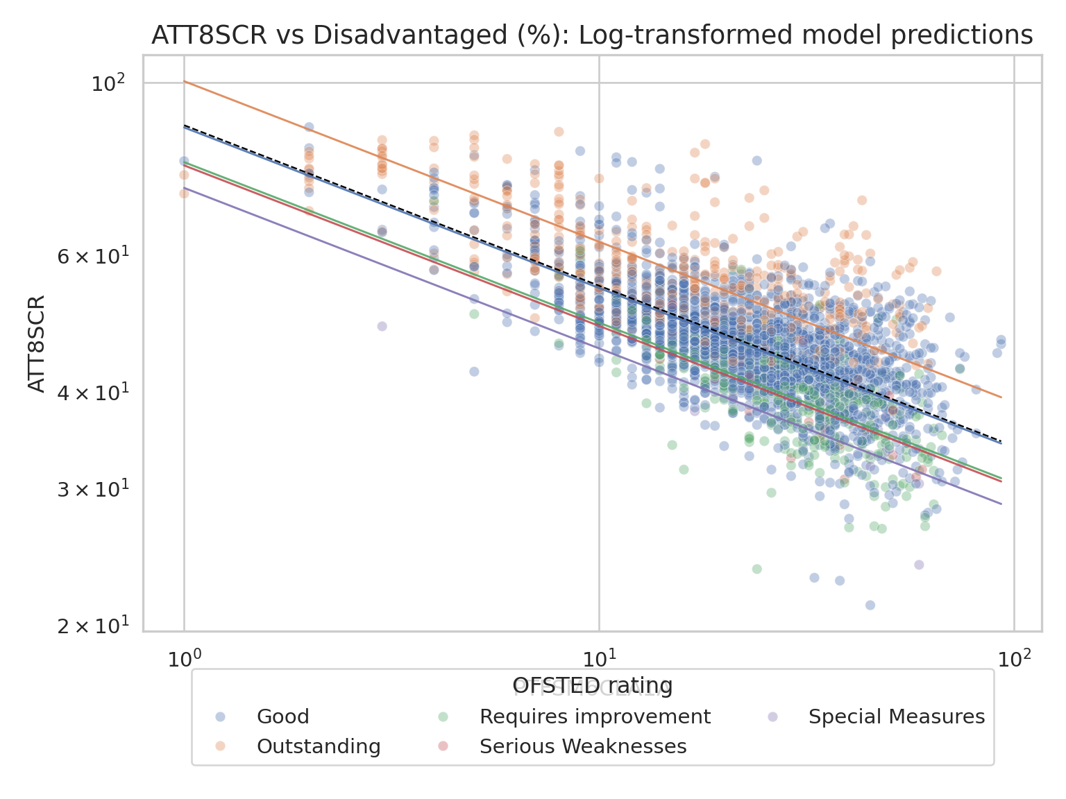
Stage 2 - Adding an initial Fixed Effect

Model with a Fixed Effect Predictor (random intercepts, fixed slopes)

In the lecture you saw that after running the null model (assuming the ICC indicates that a mixed effects model is recommended) the next stage is to test that model by adding in a predictor variable
You can use any predictor you like and once you get used to running these models, you can even skip this step, but for now we are going to build gradually and I am going to experiment with the % disadvantaged variable

Code

import pandas as pd
import numpy as np
import matplotlib.pyplot as plt
import seaborn as sns
import statsmodels.formula.api as smf

# 1. Clean data and check
df = england_filtered_clean.copy()
print("Original shape:", df.shape)

Original shape: (2961, 118)

Code

# Drop missing values
df = df.dropna(subset=["ATT8SCR", "PTFSM6CLA1A", "OFSTEDRATING"])
print("After dropna:", df.shape)

After dropna: (2902, 118)

Code

# Ensure correct types
df["OFSTEDRATING"] = df["OFSTEDRATING"].astype(str)
print("Groups:", df["OFSTEDRATING"].unique())

Groups: ['Good' 'Outstanding' 'Requires improvement' 'Serious Weaknesses'
 'Special Measures']

Code

if df.empty:
    raise ValueError("No data left after cleaning. Check column names and missing values.")

# 2. Apply log transformation
df["log_ATT8SCR"] = np.log(df["ATT8SCR"])
df["log_PTFSM6CLA1A"] = np.log(df["PTFSM6CLA1A"])

# 3. Fit simple linear model (fixed effect)
lm = smf.ols("log_ATT8SCR ~ log_PTFSM6CLA1A", data=df).fit()
fixed_intercept = lm.params["Intercept"]
slope = lm.params["log_PTFSM6CLA1A"]
print("Fixed effects:", lm.params)

Fixed effects: Intercept          4.478310
log_PTFSM6CLA1A   -0.206907
dtype: float64

Code

# 4. Compute group-specific intercept adjustments
df["residual"] = df["log_ATT8SCR"] - (fixed_intercept + slope * df["log_PTFSM6CLA1A"])
group_adjustments = df.groupby("OFSTEDRATING")["residual"].mean().reset_index()
group_adjustments.rename(columns={"residual": "blup"}, inplace=True)
print("Group adjustments:", group_adjustments)

Group adjustments:            OFSTEDRATING      blup
0                  Good -0.006606
1           Outstanding  0.130557
2  Requires improvement -0.109573
3    Serious Weaknesses -0.119260
4      Special Measures -0.185965

Code

# 5. Prediction grid (log scale)
pop_range = np.linspace(df["log_PTFSM6CLA1A"].min(), df["log_PTFSM6CLA1A"].max(), 100)

# Build predictions for each group
pred_list = []
for _, row in group_adjustments.iterrows():
    intercept_i = fixed_intercept + row["blup"]
    pred_list.append(pd.DataFrame({
        "log_PTFSM6CLA1A": pop_range,
        "log_ATT8SCR": intercept_i + slope * pop_range,
        "OFSTEDRATING": row["OFSTEDRATING"]
    }))
pred_df = pd.concat(pred_list, ignore_index=True)

# Back-transform predictions to original scale
pred_df["PTFSM6CLA1A"] = np.exp(pred_df["log_PTFSM6CLA1A"])
pred_df["ATT8SCR"] = np.exp(pred_df["log_ATT8SCR"])

# Overall line
overall_df = pd.DataFrame({
    "log_PTFSM6CLA1A": pop_range,
    "log_ATT8SCR": fixed_intercept + slope * pop_range
})
overall_df["PTFSM6CLA1A"] = np.exp(overall_df["log_PTFSM6CLA1A"])
overall_df["ATT8SCR"] = np.exp(overall_df["log_ATT8SCR"])

# 6. Plot (original scale)
sns.set_theme(style="whitegrid")
fig, ax = plt.subplots(figsize=(8, 6))

# Raw points
sns.scatterplot(
    data=df,
    x="PTFSM6CLA1A", y="ATT8SCR", hue="OFSTEDRATING",
    alpha=0.35, s=30, ax=ax
)

<Axes: xlabel='PTFSM6CLA1A', ylabel='ATT8SCR'>

Code

# Group-specific lines
sns.lineplot(
    data=pred_df,
    x="PTFSM6CLA1A", y="ATT8SCR", hue="OFSTEDRATING",
    linewidth=1.1, alpha=0.9, ax=ax, legend=False
)

<Axes: xlabel='PTFSM6CLA1A', ylabel='ATT8SCR'>

Code

# Overall line
sns.lineplot(
    data=overall_df,
    x="PTFSM6CLA1A", y="ATT8SCR",
    color="black", linestyle="--", linewidth=0.9, ax=ax
)

<Axes: xlabel='PTFSM6CLA1A', ylabel='ATT8SCR'>

Code

# Titles & labels
ax.set_title("ATT8SCR vs Disadvantaged (%): Log-transformed model predictions", fontsize=14)

Text(0.5, 1.0, 'ATT8SCR vs Disadvantaged (%): Log-transformed model predictions')

Code

ax.set_xlabel("PTFSM6CLA1A")

Text(0.5, 0, 'PTFSM6CLA1A')

Code

ax.set_ylabel("ATT8SCR")

Text(0, 0.5, 'ATT8SCR')

Code

ax.legend(title="OFSTED rating", loc="lower center", bbox_to_anchor=(0.5, -0.25), ncol=3)

<matplotlib.legend.Legend object at 0x7f2170d83cd0>

Code

ax.set_xscale("log")
ax.set_yscale("log")

plt.tight_layout()
plt.show()

Code

library(lme4)
library(ggplot2)
library(dplyr)
library(tibble)

# Fit the model
lme2 <- lmer(log(ATT8SCR) ~ log(PTFSM6CLA1A) + (1 | OFSTEDRATING), data = england_filtered_clean)

# Fixed effects
fixed_intercept <- fixef(lme2)[1]
slope <- fixef(lme2)[2]

# Random intercepts (BLUPs)
ranef_df <- ranef(lme2)$OFSTEDRATING %>%
  as.data.frame() %>%
  rownames_to_column("OFSTEDRATING") %>%
  rename(blup = `(Intercept)`)

# Prediction grid across observed range (raw values)
pop_range <- seq(
  min(england_filtered_clean$PTFSM6CLA1A, na.rm = TRUE),
  max(england_filtered_clean$PTFSM6CLA1A, na.rm = TRUE),
  length.out = 100
)

# Lines for each OFSTED group: apply log in prediction
pred_df <- do.call(rbind, lapply(seq_len(nrow(ranef_df)), function(i) {
  intercept_i <- fixed_intercept + ranef_df$blup[i]
  data.frame(
    PTFSM6CLA1A = pop_range,
    ATT8SCR = exp(intercept_i + slope * log(pop_range)),  # back-transform to original scale
    OFSTEDRATING = ranef_df$OFSTEDRATING[i],
    stringsAsFactors = FALSE
  )
}))

# Overall fixed-effects line
overall_df <- data.frame(
  PTFSM6CLA1A = pop_range,
  ATT8SCR = exp(fixed_intercept + slope * log(pop_range))  # back-transform
)

# Plot: raw points and fitted lines
ggplot() +
  geom_point(
    data = england_filtered_clean,
    aes(x = log(PTFSM6CLA1A), y = log(ATT8SCR), color = OFSTEDRATING),
    alpha = 0.35, size = 1.2, na.rm = TRUE
  ) +
  geom_line(
    data = pred_df,
    aes(x = log(PTFSM6CLA1A), y = log(ATT8SCR), color = OFSTEDRATING),
    linewidth = 1.1, alpha = 0.9
  ) +
  geom_line(
    data = overall_df,
    aes(x = log(PTFSM6CLA1A), y = log(ATT8SCR)),
    color = "black", linetype = "dashed", linewidth = 0.9
  ) +
  scale_color_brewer(palette = "Set2") +
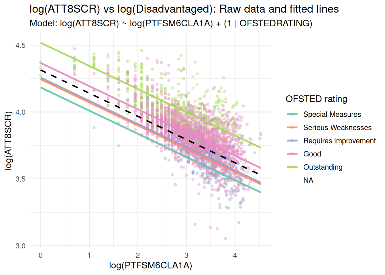
  labs(
    title = "log(ATT8SCR) vs log(Disadvantaged): Raw data and fitted lines",
    subtitle = "Model: log(ATT8SCR) ~ log(PTFSM6CLA1A) + (1 | OFSTEDRATING)",
    x = "log(PTFSM6CLA1A)",
    y = "log(ATT8SCR)",
    color = "OFSTED rating"
  ) +
  theme_minimal(base_size = 12)

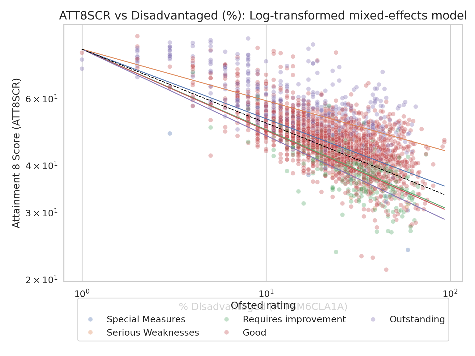
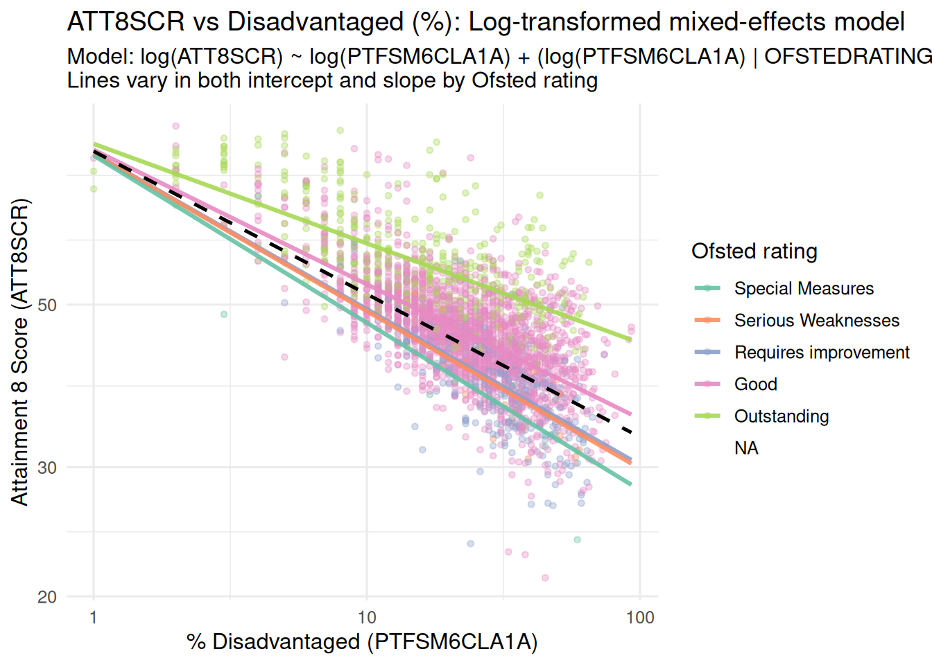
Random Intercepts and Random Slopes Model

And again, in the lecture we saw that the next stage once you have allowed your intercepts to vary, is to allow your slopes to vary as well
Here’s the visualisation of those varying slopes and intercepts:

Code

import pandas as pd
import numpy as np
import statsmodels.formula.api as smf
import matplotlib.pyplot as plt
import seaborn as sns

df = england_filtered_clean.copy()
df["log_ATT8SCR"] = np.log(df["ATT8SCR"])
df["log_PTFSM6CLA1A"] = np.log(df["PTFSM6CLA1A"])

# Drop rows with missing values in any relevant column
df = df.dropna(subset=["log_ATT8SCR", "log_PTFSM6CLA1A", "OFSTEDRATING"])

# Fit mixed model with random intercepts and slopes
model = smf.mixedlm(
    "log_ATT8SCR ~ log_PTFSM6CLA1A",
    df,
    groups=df["OFSTEDRATING"],
    re_formula="~log_PTFSM6CLA1A"
)
lme_rs = model.fit(reml=False, method="lbfgs")

/opt/hostedtoolcache/Python/3.10.19/x64/lib/python3.10/site-packages/statsmodels/regression/mixed_linear_model.py:2237: ConvergenceWarning: The MLE may be on the boundary of the parameter space.
  warnings.warn(msg, ConvergenceWarning)
/opt/hostedtoolcache/Python/3.10.19/x64/lib/python3.10/site-packages/statsmodels/regression/mixed_linear_model.py:2261: ConvergenceWarning: The Hessian matrix at the estimated parameter values is not positive definite.
  warnings.warn(msg, ConvergenceWarning)

Code

# Fixed effects
fixed_intercept = lme_rs.fe_params["Intercept"]
fixed_slope = lme_rs.fe_params["log_PTFSM6CLA1A"]

# Random effects per group (intercept and slope deviations)
ranef = lme_rs.random_effects
re_df = pd.DataFrame([
    {
        "OFSTEDRATING": g,
        "b0": v.get("Intercept", v.get("0", 0)),  # intercept deviation
        "b1": v.get("log_PTFSM6CLA1A", 0)         # slope deviation
    }
    for g, v in ranef.items()
])

# Prediction grid (log scale)
x_range_log = np.linspace(np.log(df["PTFSM6CLA1A"].min()), np.log(df["PTFSM6CLA1A"].max()), 100)

# Build predictions for each group
pred_list = []
for _, row in re_df.iterrows():
    intercept_i = fixed_intercept + row["b0"]
    slope_i = fixed_slope + row["b1"]
    pred_list.append(pd.DataFrame({
        "OFSTEDRATING": row["OFSTEDRATING"],
        "PTFSM6CLA1A": np.exp(x_range_log),
        "ATT8SCR": np.exp(intercept_i + slope_i * x_range_log)
    }))
pred_df = pd.concat(pred_list)

# Overall fixed-effects line
overall_df = pd.DataFrame({
    "PTFSM6CLA1A": np.exp(x_range_log),
    "ATT8SCR": np.exp(fixed_intercept + fixed_slope * x_range_log)
})

# Plot
sns.set_theme(style="whitegrid")
fig, ax = plt.subplots(figsize=(8, 6))

sns.scatterplot(data=df, x="PTFSM6CLA1A", y="ATT8SCR", hue="OFSTEDRATING", alpha=0.35, s=30, ax=ax)

<Axes: xlabel='PTFSM6CLA1A', ylabel='ATT8SCR'>

Code

sns.lineplot(data=pred_df, x="PTFSM6CLA1A", y="ATT8SCR", hue="OFSTEDRATING", linewidth=1.1, alpha=0.9, ax=ax, legend=False)

<Axes: xlabel='PTFSM6CLA1A', ylabel='ATT8SCR'>

Code

sns.lineplot(data=overall_df, x="PTFSM6CLA1A", y="ATT8SCR", color="black", linestyle="--", linewidth=0.9, ax=ax)

<Axes: xlabel='PTFSM6CLA1A', ylabel='ATT8SCR'>

Code

ax.set_xscale("log")
ax.set_yscale("log")
ax.set_title("ATT8SCR vs Disadvantaged (%): Log-transformed mixed-effects model", fontsize=14)

Text(0.5, 1.0, 'ATT8SCR vs Disadvantaged (%): Log-transformed mixed-effects model')

Code

ax.set_xlabel("% Disadvantaged (PTFSM6CLA1A)")

Text(0.5, 0, '% Disadvantaged (PTFSM6CLA1A)')

Code

ax.set_ylabel("Attainment 8 Score (ATT8SCR)")

Text(0, 0.5, 'Attainment 8 Score (ATT8SCR)')

Code

ax.legend(title="Ofsted rating", loc="lower center", bbox_to_anchor=(0.5, -0.25), ncol=3)

<matplotlib.legend.Legend object at 0x7f21709080d0>

Code

plt.tight_layout()
plt.show()

Code

# Packages
library(lme4)
library(ggplot2)
library(dplyr)
library(tibble)

# --- Prepare log-transformed variables
england_filtered_clean <- england_filtered_clean %>%
  mutate(
    log_ATT8SCR = log(ATT8SCR),
    log_PTFSM6CLA1A = log(PTFSM6CLA1A)
  )

# --- Fit random intercept + random slope model
lme_rs <- lmer(log_ATT8SCR ~ log_PTFSM6CLA1A + (log_PTFSM6CLA1A | OFSTEDRATING),
               data = england_filtered_clean)

# Fixed effects
fixed_intercept <- fixef(lme_rs)[["(Intercept)"]]
fixed_slope     <- fixef(lme_rs)[["log_PTFSM6CLA1A"]]

# Random effects (BLUPs) per group: intercept and slope
re_df <- ranef(lme_rs)$OFSTEDRATING %>%
  rownames_to_column("OFSTEDRATING") %>%
  rename(
    b0 = `(Intercept)`,          # random intercept deviation
    b1 = `log_PTFSM6CLA1A`       # random slope deviation
  )

# Prediction grid across observed range (log scale)
x_range_log <- seq(
  min(log(england_filtered_clean$PTFSM6CLA1A), na.rm = TRUE),
  max(log(england_filtered_clean$PTFSM6CLA1A), na.rm = TRUE),
  length.out = 100
)

# Build per-group prediction lines (varying intercepts & slopes)
pred_df <- do.call(rbind, lapply(seq_len(nrow(re_df)), function(i) {
  intercept_i <- fixed_intercept + re_df$b0[i]
  slope_i     <- fixed_slope     + re_df$b1[i]
  data.frame(
    OFSTEDRATING = re_df$OFSTEDRATING[i],
    PTFSM6CLA1A  = exp(x_range_log),
    ATT8SCR      = exp(intercept_i + slope_i * x_range_log),
    stringsAsFactors = FALSE
  )
}))

# Overall fixed-effects line
overall_df <- data.frame(
  PTFSM6CLA1A = exp(x_range_log),
  ATT8SCR     = exp(fixed_intercept + fixed_slope * x_range_log)
)

# --- Plot: raw data + group-specific fitted lines
ggplot() +
  # Raw points
  geom_point(
    data = england_filtered_clean,
    aes(x = PTFSM6CLA1A, y = ATT8SCR, color = OFSTEDRATING),
    alpha = 0.35, size = 1.2, na.rm = TRUE
  ) +
  # Group-specific lines
  geom_line(
    data = pred_df,
    aes(x = PTFSM6CLA1A, y = ATT8SCR, color = OFSTEDRATING),
    linewidth = 1.1, alpha = 0.9
  ) +
  # Overall line
  geom_line(
    data = overall_df,
    aes(x = PTFSM6CLA1A, y = ATT8SCR),
    color = "black", linetype = "dashed", linewidth = 0.9
  ) +
  scale_color_brewer(palette = "Set2", name = "Ofsted rating") +
  scale_x_log10() +
  scale_y_log10() +
  labs(
    title = "ATT8SCR vs Disadvantaged (%): Log-transformed mixed-effects model",
    subtitle = "Model: log(ATT8SCR) ~ log(PTFSM6CLA1A) + (log(PTFSM6CLA1A) | OFSTEDRATING)\nLines vary in both intercept and slope by Ofsted rating",
    x = "% Disadvantaged (PTFSM6CLA1A)",
    y = "Attainment 8 Score (ATT8SCR)"
  ) +
  theme_minimal(base_size = 12)

Fitting a Basic Random Effect and Random Slope Model

And now we can also fit the model using statistical software

Code

import pandas as pd
import statsmodels.formula.api as smf

df_clean = df.dropna(subset=["log_ATT8SCR", "log_PTFSM6CLA1A", "OFSTEDRATING"])

# Example
model = smf.mixedlm(
    "log_ATT8SCR ~ log_PTFSM6CLA1A",
    data=df_clean,
    groups=df_clean["OFSTEDRATING"],
    re_formula="~log_PTFSM6CLA1A"
)

result = model.fit()

/opt/hostedtoolcache/Python/3.10.19/x64/lib/python3.10/site-packages/statsmodels/base/model.py:607: ConvergenceWarning: Maximum Likelihood optimization failed to converge. Check mle_retvals
  warnings.warn("Maximum Likelihood optimization failed to "
/opt/hostedtoolcache/Python/3.10.19/x64/lib/python3.10/site-packages/statsmodels/regression/mixed_linear_model.py:2200: ConvergenceWarning: Retrying MixedLM optimization with lbfgs
  warnings.warn(
/opt/hostedtoolcache/Python/3.10.19/x64/lib/python3.10/site-packages/statsmodels/base/model.py:607: ConvergenceWarning: Maximum Likelihood optimization failed to converge. Check mle_retvals
  warnings.warn("Maximum Likelihood optimization failed to "
/opt/hostedtoolcache/Python/3.10.19/x64/lib/python3.10/site-packages/statsmodels/regression/mixed_linear_model.py:2200: ConvergenceWarning: Retrying MixedLM optimization with cg
  warnings.warn(
/opt/hostedtoolcache/Python/3.10.19/x64/lib/python3.10/site-packages/statsmodels/base/model.py:607: ConvergenceWarning: Maximum Likelihood optimization failed to converge. Check mle_retvals
  warnings.warn("Maximum Likelihood optimization failed to "
/opt/hostedtoolcache/Python/3.10.19/x64/lib/python3.10/site-packages/statsmodels/regression/mixed_linear_model.py:2206: ConvergenceWarning: MixedLM optimization failed, trying a different optimizer may help.
  warnings.warn(msg, ConvergenceWarning)
/opt/hostedtoolcache/Python/3.10.19/x64/lib/python3.10/site-packages/statsmodels/regression/mixed_linear_model.py:2218: ConvergenceWarning: Gradient optimization failed, |grad| = 18.082090
  warnings.warn(msg, ConvergenceWarning)
/opt/hostedtoolcache/Python/3.10.19/x64/lib/python3.10/site-packages/statsmodels/regression/mixed_linear_model.py:2237: ConvergenceWarning: The MLE may be on the boundary of the parameter space.
  warnings.warn(msg, ConvergenceWarning)

Code

print(result.summary())

                 Mixed Linear Model Regression Results
=======================================================================
Model:                  MixedLM     Dependent Variable:     log_ATT8SCR
No. Observations:       2902        Method:                 REML       
No. Groups:             5           Scale:                  0.0141     
Min. group size:        16          Log-Likelihood:         2047.0001  
Max. group size:        2076        Converged:              No         
Mean group size:        580.4                                          
-----------------------------------------------------------------------
                            Coef.  Std.Err.    z    P>|z| [0.025 0.975]
-----------------------------------------------------------------------
Intercept                    4.400    0.037 117.605 0.000  4.327  4.473
log_PTFSM6CLA1A             -0.196    0.017 -11.789 0.000 -0.229 -0.164
Group Var                    0.002                                     
Group x log_PTFSM6CLA1A Cov -0.001                                     
log_PTFSM6CLA1A Var          0.001    0.004                            
=======================================================================

Code

lme3 <- lmer(log(ATT8SCR) ~ log(PTFSM6CLA1A) + (log(PTFSM6CLA1A)|OFSTEDRATING), data = england_filtered_clean)

boundary (singular) fit: see help('isSingular')

Code

summary(lme3)

Linear mixed model fit by REML ['lmerMod']
Formula: log(ATT8SCR) ~ log(PTFSM6CLA1A) + (log(PTFSM6CLA1A) | OFSTEDRATING)
   Data: england_filtered_clean

REML criterion at convergence: -4098.3

Scaled residuals: 
    Min      1Q  Median      3Q     Max 
-5.4441 -0.6172 -0.0349  0.5795  4.7032 

Random effects:
 Groups       Name             Variance  Std.Dev. Corr
 OFSTEDRATING (Intercept)      0.0002147 0.01465      
              log(PTFSM6CLA1A) 0.0013767 0.03710  1.00
 Residual                      0.0140766 0.11864      
Number of obs: 2902, groups:  OFSTEDRATING, 5

Fixed effects:
                 Estimate Std. Error t value
(Intercept)       4.39367    0.01319  333.12
log(PTFSM6CLA1A) -0.19491    0.01707  -11.42

Correlation of Fixed Effects:
            (Intr)
l(PTFSM6CLA 0.315 
optimizer (nloptwrap) convergence code: 0 (OK)
boundary (singular) fit: see help('isSingular')

Interpretation

NB - this applies to these models above, you will have different interpretations depending on the variables you have chosen

Here we have fitted a basic random intercept and random slope model using comparable methods in R and Python.

Fixed Effects

Intercept (≈ 4.39) This is the expected value of log(ATT8SCR) when log(PTFSM6CLA1A) is zero (i.e., when the predictor is at its baseline). In practical terms, it’s the average log score for schools at the reference level of the predictor.

Slope for log(PTFSM6CLA1A) (≈ −0.195) For each 1-unit increase in the log of PTFSM6CLA1A, the log of ATT8SCR decreases by about 0.195. Since both variables are logged, this is roughly an elasticity: higher PTFSM6CLA1A is associated with lower ATT8SCR.

Random Effects

OFSTEDRATING intercept variance (≈ 0.00021) There’s very little variation in baseline performance across OFSTED categories after accounting for the fixed effect.

Random slope variance (≈ 0.00138) The effect of log(PTFSM6CLA1A) barely varies by OFSTED category—almost zero. The correlation between intercept and slope is estimated as 1.00, which is why you see the “singular fit” warning (R) and Convergence Warnings in Python: the model is on the boundary, meaning the random slope is not really supported by the data.

Residual variance (≈ 0.014) This is the within-group variability not explained by the model.

Experimenting with your own linear mixed effects models

At this point, this is about all you need to know, for now, to run your own linear mixed effects model.

In general you might find it’s a bit easier to run these models in R using the lme4 package, however, there are Python Packages that allow you to run linear mixed effects models using R-like syntax like Pymer4.

Please experiment - I was running into problems with Pymer4 in this practical, so you might need to persevere a bit if you want to persist on the Python track.

Pymer4 - https://eshinjolly.com/pymer4/

lme4 - https://github.com/lme4/lme4/

I didn’t touch on the Bayesian versions of these models either (a world that would have taken us many more weeks to get into!). But you can run Bayesian Linear Mixed Effects models too and there are packages in both R and Python to do this.

In Python you have bambi - https://bambinos.github.io/bambi/

In R you have RStan - https://mc-stan.org/rstan/index.html

If you remember from the lecture, there are a range of variations on the basic model which may or may not be appropriate in different situations. I’ll reproduce the table below:

Element	Meaning	Sample Equation
`(1\|g)`	Null Model or Varying Intercept Model	`P8 ~ 1 + (1 \| OFSTEDRATING)`
`(1\|g1/g2)`	Multilevel Model with intercept varying within g1 and for g2 within g1	`P8 ~ 1 + (1 \| LocalAuthority/Region)`
`(1\|g1) + (1\|g2)`	Intercept varying among g1 and g2	`P8 ~ 1 + (1 \| OFSTEDRATING) + (1 \| Region)`
`(0+x\|g)`	Varying Slope Model	`P8 ~ Disadvantage + (0 + Disadvantage \| OFSTEDRATING)`
`x + (x\|g)`	Varying and correlated intercepts and slopes	`P8 ~ Disadvantage + (Disadvantage \| OFSTEDRATING)`
`x + (x\|\|g)`	Uncorrelated Intercepts and Slopes	`P8 ~ Disadvantage + (Disadvantage \|\| OFSTEDRATING)`

You might want to experiment with only one or two of these linear mixed effects models. Below you will see I have incorporated both multilevel (local authorities nested within regions) and varying intercepts. There are almost infinite combinations.

Final Task

You should try and extend your final multiple regression showstopper model to incorporate one or more logical random effect. What can you say about the random effects in your model?
I have played around with a few additional variables too, you don’t have to do this, but you can if you wish.

My final mixed effects model

Code

#Sorry, I really tried to get this working properly with pymer, but I couldn't - too much pain. 

# Try the R version instead, or, if you manage to get as far as getting pymer4 to work, you can translate my model below into pymer4 syntax (as it uses R under the hood)

Code

lme11 <- lmer(
  log(ATT8SCR) ~ log(PTFSM6CLA1A) + log(PERCTOT) + log(PNUMEAL) +
    PTPRIORLO + ADMPOL_PT + gorard_segregation +
    log(remained_in_the_same_school) + teachers_on_leadership_pay_range_percent + log(average_number_of_days_taken.x) + 
    (1 | OFSTEDRATING) + (1 | gor_name/LANAME),
  data = england_filtered_clean,
  na.action = na.exclude
)

summary(lme11)

Linear mixed model fit by REML ['lmerMod']
Formula: log(ATT8SCR) ~ log(PTFSM6CLA1A) + log(PERCTOT) + log(PNUMEAL) +  
    PTPRIORLO + ADMPOL_PT + gorard_segregation + log(remained_in_the_same_school) +  
    teachers_on_leadership_pay_range_percent + log(average_number_of_days_taken.x) +  
    (1 | OFSTEDRATING) + (1 | gor_name/LANAME)
   Data: england_filtered_clean

REML criterion at convergence: -6621.5

Scaled residuals: 
    Min      1Q  Median      3Q     Max 
-5.5124 -0.5829  0.0062  0.6573  3.5098 

Random effects:
 Groups          Name        Variance  Std.Dev.
 LANAME:gor_name (Intercept) 0.0006629 0.02575 
 gor_name        (Intercept) 0.0002362 0.01537 
 OFSTEDRATING    (Intercept) 0.0026148 0.05114 
 Residual                    0.0047094 0.06862 
Number of obs: 2746, groups:  
LANAME:gor_name, 151; gor_name, 9; OFSTEDRATING, 5

Fixed effects:
                                           Estimate Std. Error t value
(Intercept)                               4.5645271  0.0376270 121.310
log(PTFSM6CLA1A)                         -0.0692973  0.0040523 -17.101
log(PERCTOT)                             -0.2174420  0.0076026 -28.601
log(PNUMEAL)                              0.0132556  0.0017721   7.480
PTPRIORLO                                -0.0063902  0.0002244 -28.477
ADMPOL_PTOTHER NON SEL                    0.0050957  0.0088441   0.576
ADMPOL_PTSEL                              0.0876679  0.0097675   8.975
gorard_segregation                       -0.0270332  0.0717587  -0.377
log(remained_in_the_same_school)          0.0235350  0.0036604   6.430
teachers_on_leadership_pay_range_percent -0.0009734  0.0003218  -3.025
log(average_number_of_days_taken.x)      -0.0205674  0.0036548  -5.628

Correlation of Fixed Effects:
            (Intr) l(PTFS l(PERC l(PNUM PTPRIO ADMPNS ADMPOL grrd_s l(____)
l(PTFSM6CLA -0.166                                                         
lg(PERCTOT) -0.313 -0.347                                                  
lg(PNUMEAL) -0.025 -0.266  0.163                                           
PTPRIORLO    0.037 -0.366 -0.198 -0.162                                    
ADMPOL_PTNS -0.223 -0.045  0.027 -0.014  0.075                             
ADMPOL_PTSE -0.308  0.197  0.034 -0.228  0.308  0.548                      
grrd_sgrgtn -0.333  0.139 -0.067  0.024 -0.024 -0.026  0.026               
lg(rmn____) -0.503  0.108  0.041 -0.114  0.146  0.017  0.182  0.058        
tchrs_n____ -0.229 -0.091  0.024 -0.007 -0.040 -0.008  0.020  0.035  0.361 
lg(vr____.) -0.156 -0.015 -0.132 -0.013 -0.004 -0.008 -0.001  0.030  0.031 
            t_____
l(PTFSM6CLA       
lg(PERCTOT)       
lg(PNUMEAL)       
PTPRIORLO         
ADMPOL_PTNS       
ADMPOL_PTSE       
grrd_sgrgtn       
lg(rmn____)       
tchrs_n____       
lg(vr____.)  0.021

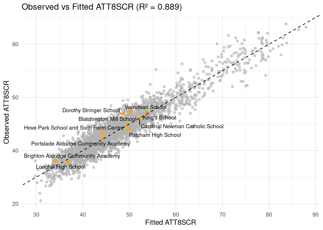
Fitted Values vs Observed Attainment 8 (how good is the model?)

Here I have overlaid the Brighton Schools again - anything above the line (a positive residual) shows the school is doing better than expected, given the variables we have used to predict attainment. Anything below, the school is performing worse than expected.

Code

# Add fitted values (back-transform to original scale)
england_filtered_clean <- england_filtered_clean %>%
  mutate(fitted_ATT8SCR = exp(fitted(lme11)))

# Compute R²
r2 <- cor(england_filtered_clean$ATT8SCR, england_filtered_clean$fitted_ATT8SCR, use = "complete.obs")^2

# Identify Brighton schools
brighton_schools <- england_filtered_clean %>%
  filter(LANAME == "Brighton and Hove")

# Plot
ggplot(england_filtered_clean, aes(x = fitted_ATT8SCR, y = ATT8SCR)) +
  geom_point(color = "grey70", alpha = 0.6) +
  geom_point(data = brighton_schools, color = "orange", size = 2) +
  geom_text_repel(data = brighton_schools,
                  aes(label = SCHNAME.x),
                  color = "black",
                  size = 3,
                  max.overlaps = 20) +
  geom_abline(slope = 1, intercept = 0, linetype = "dashed", color = "black") +
  labs(
    title = paste0("Observed vs Fitted ATT8SCR (R² = ", round(r2, 3), ")"),
    x = "Fitted ATT8SCR",
    y = "Observed ATT8SCR"
  ) +
  theme_minimal()

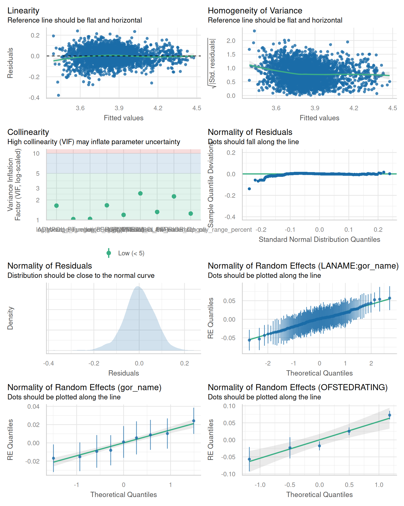
Warning: Removed 7 rows containing missing values or values outside the scale range
(`geom_point()`).

We can also run some diagnostic plots to double check our model adheres to the various assumptions required

Code

library(performance)
check_model(lme11)

Interpreting your outputs

Random Effects

Turning the Std.Dev to an approximate percentage difference: \(\%= 100 \times (exp(SD) - 1)\). This gives a feel for how much Attainment 8 changes for a +1 SD higher group intercept.

lme11 (Overall Attainment 8)

OFSTEDRATING: Var = 0.0026, SD = 0.051 → ~+5.2% per +1 SD
Region (gor_name): Var = 0.00024, SD = 0.015 → ~+1.5%
LA within Region: Var = 0.00066, SD = 0.026 → ~+2.6%
Residual (school-level/unexplained): Var = 0.00471, SD = 0.069 → ~+7.1%

Taking the sum of all the variances and dividing each individual variance by this total gives the proportion of variance explained by each random effect:

OFSTEDRATING: 31.8%
Region: 2.9%
LA within Region: 8.1%
Residual: 57.3%
Total variance: 0.00822

While Ofsted Rating helps explain a lot of the variance - some 32%, most of the variability is between individual schools within each group.

Fixed Effects

From lme11 (overall attainment):

Most influential negative factors:
- Overall absence (log(PERCTOT)): t ≈ -28.6 → Higher absence strongly reduces attainment.
- Prior low attainment (PTPRIORLO): t ≈ -28.5 → Schools with more students entering low-performing do worse.
- Proportion disadvantaged (log(PTFSM6CLA1A)): t ≈ -17.1 → Higher concentration of disadvantaged pupils lowers overall attainment, but is much less important than the first two factors.
Positive factors:
- Selective admissions (ADMPOL_PTSEL): t ≈ 9.0 → Selective schools boost attainment.
- Proportion EAL (log(PNUMEAL)): t ≈ 7.5 → Linguistic diversity slightly improves outcomes.
- Teacher Stability (log(remained_in_the_same_school)): t ≈ 6.4 → Teachers remaining in the same school helps.
Moderate negatives:
- Teacher Absence days: t ≈ -5.6.
- Proportion of Teachers on Leadership pay %: t ≈ -3.0.
Not significant: Other admission policy, segregation index.

Overall Fit

Comparing the Observed and Fitted Values and calculating an \(R^2\) value from that, we can explain almost 90% of the variation in Attainment 8. Schools in Brighton are mainly showing positive residuals - in other words, performing much better than other similar schools in England with similar profiles.

Benefits of LME over OLS

Accounts for clustering (schools within OFSTED/regions).

Shrinkage / “Partial pooling” reduces overfitting and improves predictions.

Decomposes variance across levels so we can see how, for example, having a better Ofsted score might compare with lowering absence.

School-specific predictions are more useful.

Policy Interpretations and Using AI to help with the specific, contextual translation of outputs

Below I have pulled out some of the schools in Brighton.
One of the nice things about AI is it is very good at quickly turning specific situations into policy-relevant examples using the models we have just built. Have a look at the table below and I will give you an example of a question that produces some very interesting results:

Code

# Packages
library(dplyr)
library(tidyr)
library(stringr)
library(lme4)
library(tibble)

# --- Schools of interest ---
target_urns  <- c("114581", "14608", "136164", "114580")
target_names <- c("Longhill High School", "Patcham High School", "Brighton Aldridge Community Academy", "Dorothy Stringer School")

# --- Variables of interest (from your final model) ---
vars_of_interest <- c(
  "PERCTOT",        # % overall absence
  "PTFSM6CLA1A",    # % disadvantaged
  "PNUMEAL",        # cohort size proxy
  "PTPRIORLO",      # prior low attainment
  "ADMPOL_PT",      # admissions policy
  "gorard_segregation", # LA-level segregation
  "remained_in_the_same_school",   # total teachers remained_in_the_same_school
  "teachers_on_leadership_pay_range_percent", # leadership pay %
  "average_number_of_days_taken.x"  # average sick days
)

# 1) Subset to target schools
schools_sub <- england_filtered_clean %>%
  filter(URN %in% target_urns | SCHNAME.x %in% target_names) %>%
  select(URN, SCHNAME.x, OFSTEDRATING, gor_name, LANAME, all_of(vars_of_interest)) %>%
  distinct()

# 2) Extract random effects from lme11
re_list <- lme4::ranef(lme11)

# 2a) OFSTEDRATING random intercepts
re_ofsted <- re_list$OFSTEDRATING %>%
  as.data.frame() %>%
  rownames_to_column("OFSTEDRATING") %>%
  rename(re_OFSTEDRATING = `(Intercept)`)

# 2b) gor_name random intercepts
re_gor <- re_list$gor_name %>%
  as.data.frame() %>%
  rownames_to_column("gor_name") %>%
  rename(re_gor_name = `(Intercept)`)

# 2c) Nested random intercepts for LANAME:gor_name
grp_names <- names(re_list)
lan_gor_grp <- grp_names[grepl("LANAME.*gor_name|gor_name.*LANAME", grp_names)][1]

if (grepl("^LANAME", lan_gor_grp)) {
  re_lan_gor <- re_list[[lan_gor_grp]] %>%
    as.data.frame() %>%
    rownames_to_column("key") %>%
    separate(key, into = c("LANAME", "gor_name"), sep = ":", remove = TRUE) %>%
    rename(re_LANAME_gor = `(Intercept)`)
} else {
  re_lan_gor <- re_list[[lan_gor_grp]] %>%
    as.data.frame() %>%
    rownames_to_column("key") %>%
    separate(key, into = c("gor_name", "LANAME"), sep = ":", remove = TRUE) %>%
    rename(re_LANAME_gor = `(Intercept)`) %>%
    relocate(LANAME, gor_name)
}

# 3) Join random effects and compute total RE
schools_with_re <- schools_sub %>%
  left_join(re_ofsted, by = "OFSTEDRATING") %>%
  left_join(re_gor, by = "gor_name") %>%
  left_join(re_lan_gor, by = c("LANAME", "gor_name")) %>%
  mutate(RE_total = re_OFSTEDRATING + re_gor_name + re_LANAME_gor)

# 4) Predictions (log scale -> back-transform)
pred_log_fixed <- predict(lme11, newdata = schools_with_re, re.form = NA)
pred_log_cond  <- predict(lme11, newdata = schools_with_re, re.form = NULL)

# Bias correction
sigma2 <- sigma(lme11)^2
bias_factor <- exp(0.5 * sigma2)

schools_with_re <- schools_with_re %>%
  mutate(
    pred_fixed   = exp(pred_log_fixed),
    pred_cond    = exp(pred_log_cond),
    pred_cond_bc = pred_cond * bias_factor
  )

# 5) Display table
row_order <- c(
  "PERCTOT", "PTFSM6CLA1A", "PNUMEAL", "PTPRIORLO", "ADMPOL_PT",
  "gorard_segregation", "remained_in_the_same_school", "teachers_on_leadership_pay_range_percent", "average_number_of_days_taken.x",
  "RE: OFSTEDRATING", "RE: gor_name", "RE: LANAME:gor_name", "RE: total",
  "Baseline ATT8 (fixed only)", "Baseline ATT8 (incl. RE)", "Baseline ATT8 (incl. RE, bias-corrected)"
)

display_tbl <- schools_with_re %>%
  transmute(
    SCHNAME.x,
    PERCTOT = formatC(PERCTOT, format = "f", digits = 1),
    PTFSM6CLA1A = formatC(PTFSM6CLA1A, format = "f", digits = 1),
    PNUMEAL = formatC(PNUMEAL, format = "f", digits = 1),
    PTPRIORLO = formatC(PTPRIORLO, format = "f", digits = 1),
    ADMPOL_PT = as.character(ADMPOL_PT),
    gorard_segregation = formatC(gorard_segregation, format = "f", digits = 3),
    remained_in_the_same_school = formatC(remained_in_the_same_school, format = "f", digits = 3),
    teachers_on_leadership_pay_range_percent = formatC(teachers_on_leadership_pay_range_percent, format = "f", digits = 1),
    average_number_of_days_taken.x = formatC(average_number_of_days_taken.x, format = "f", digits = 3),
    `RE: OFSTEDRATING` = formatC(re_OFSTEDRATING, format = "f", digits = 3),
    `RE: gor_name` = formatC(re_gor_name, format = "f", digits = 3),
    `RE: LANAME:gor_name` = formatC(re_LANAME_gor, format = "f", digits = 3),
    `RE: total` = formatC(RE_total, format = "f", digits = 3),
    `Baseline ATT8 (fixed only)` = formatC(pred_fixed, format = "f", digits = 1),
    `Baseline ATT8 (incl. RE)` = formatC(pred_cond, format = "f", digits = 1),
    `Baseline ATT8 (incl. RE, bias-corrected)` = formatC(pred_cond_bc, format = "f", digits = 1)
  ) %>%
  pivot_longer(cols = -SCHNAME.x, names_to = "Variable", values_to = "Value") %>%
  pivot_wider(names_from = SCHNAME.x, values_from = Value) %>%
  mutate(Variable = factor(Variable, levels = row_order)) %>%
  arrange(Variable)


knitr::kable(
  display_tbl %>% arrange(Variable),
  align = "l"
)

Variable	Brighton Aldridge Community Academy	Dorothy Stringer School	Longhill High School	Patcham High School
PERCTOT	16.2	9.5	13.4	9.2
PTFSM6CLA1A	45.0	18.0	29.0	19.0
PNUMEAL	12.3	7.4	7.9	6.4
PTPRIORLO	37.0	17.0	34.0	14.0
ADMPOL_PT	OTHER NON SEL	OTHER NON SEL	OTHER NON SEL	OTHER NON SEL
gorard_segregation	0.133	0.133	0.133	0.133
remained_in_the_same_school	35.000	87.500	38.100	50.800
teachers_on_leadership_pay_range_percent	14.0	8.3	11.7	7.1
average_number_of_days_taken.x	6.000	11.800	9.700	5.900
RE: OFSTEDRATING	-0.018	0.025	-0.018	0.025
RE: gor_name	-0.015	-0.015	-0.015	-0.015
RE: LANAME:gor_name	0.035	0.035	0.035	0.035
RE: total	0.002	0.045	0.002	0.045
Baseline ATT8 (fixed only)	34.0	46.5	36.8	47.6
Baseline ATT8 (incl. RE)	34.1	48.7	36.9	49.8
Baseline ATT8 (incl. RE, bias-corrected)	34.2	48.8	37.0	49.9

Question for my AI

Given the outputs from the model above and the specific detail the variables for each school. Considering Longhill and Patcham schools, can you show what percentage point change would be required for each variable to affect an increase of 5 more Attainment 8 points?

Variable	Change (unit)	Longhill Current	Longhill Required Δ	Patcham Current	Patcham Required Δ
PERCTOT (overall absence) (log)	pp	13.4	−5.9 pp	9.2	−3.3 pp
PTFSM6CLA1A (% disadvantaged) (log)	pp	29.0	−24.3 pp	19.0	−14.2 pp

This output is highly illustrative and shows that given the different starting points for each school, not only are different levels of effort required to reach the same outcomes (Patcham would need to reduce absence by fewer percentage points to achieve the same 5 point attainment 8 increase), but we can see how much more effective reducing absence is than reducing levels of disadvantage - with Longhill needing to reduce its levels of disadvantaged students down from 29% to to 5% to achieve the same point score improvement.

Given the policy levers that Brighton and Hove Council tried to pull, this is very important information.

Task

See if you can experiment with feeding your own tame AI (Copilot/Chat GPT, ClaudeAI, Gemini etc. will all do this slightly differently and with greater or lesser success) with your model outputs and some specifics about some schools or local authorities, and then ask some questions of it to aid in some insightful interpretation.

Caution

I shouldn’t need to tell you to proceed with caution when asking an AI to interpret your outputs. It will get things wrong so don’t just copy and paste! Interrogate, ask follow-up questions. Ask for reinterpretations or to explain specific features.

Extension Activities

I think you’ve probably had enough at this point, but you will hopefully find many uses for these models in your future work.

Element	Meaning	Sample Equation
`(1\|g)`	Null Model or Varying Intercept Model	`P8 ~ 1 + (1 \| OFSTEDRATING)`
`(1\|g1/g2)`	Multilevel Model with intercept varying within g1 and for g2 within g1	`P8 ~ 1 + (1 \| LocalAuthority/Region)`
`(1\|g1) + (1\|g2)`	Intercept varying among g1 and g2	`P8 ~ 1 + (1 \| OFSTEDRATING) + (1 \| Region)`
`(0+x\|g)`	Varying Slope Model	`P8 ~ Disadvantage + (0 + Disadvantage \| OFSTEDRATING)`
`x + (x\|g)`	Varying and correlated intercepts and slopes	`P8 ~ Disadvantage + (Disadvantage \| OFSTEDRATING)`
`x + (x\|\|g)`	Uncorrelated Intercepts and Slopes	`P8 ~ Disadvantage + (Disadvantage \|\| OFSTEDRATING)`