Prof D’s Regression Sessions - Vol 3
In the mix - the linear mix(ed effects model lecture)
Adam Dennett - a.dennett@ucl.ac.uk
1st August 2024
CASA0007 Quantitative Methods
This week
Another long lecture - sorry!!
I’ll try and stop for another break in the middle
Recap
- Last week we saw how multiple regression models can allow us to understand complex relationships between predictor and outcome variables
- We began to explore how by increasing the complexity of our regression models, we can begin to observe how the effects of different variables can confound (obscure) and mediate (partially cause) the effects of others, giving us a deeper understanding of our system of interest
- We were able to see that with just a relatively small number of variables, we could explain most of the variation in school-level attainment scores in England
OLS regression with interaction terms
- In our most sophisticated model we could even see how the relationship between our main predictor and our outcome might vary between levels of a categorical variable
OLS regression with Interaction Terms
- Interacting categorical variables with other continuous predictor variables allowed us to see how levels of continuous predictor slope coefficient vary according to the categorical predictor
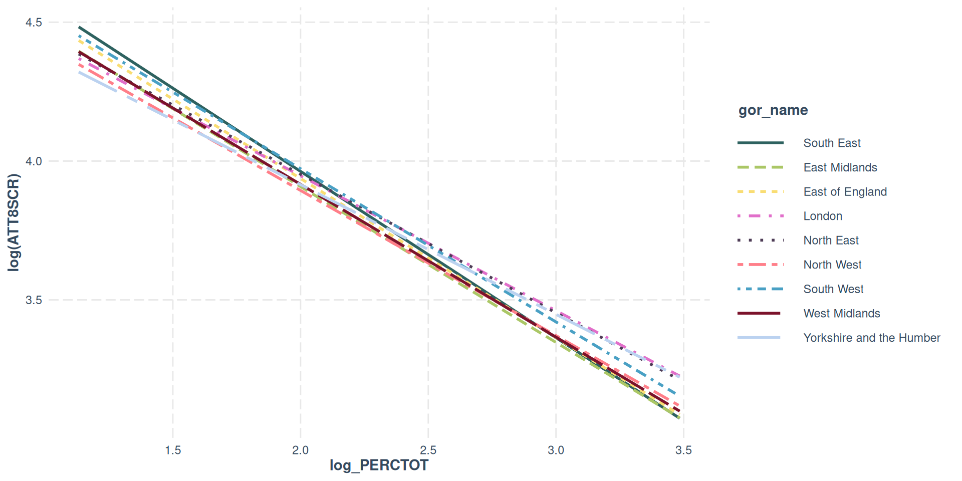
- In our example, we saw how in a simple bivariate model of Attainment 8 vs Disadvantage, the slope less severe in regions such as London, the West Midlands and Yorkshire and the Humber when compared to the South East.
- The effects of concentrations of disadvantaged pupils in schools felt more severely in the South East.
Drawbacks of OLS with Interaction
- OLS assumes all observations (schools) are independent of each other
- In reality, they may have characteristics which mean they are not independent - i.e. Being in the same local authority or having similar Ofsted ratings could mean that effects are clustered.
- OLS assumes the effects (parameters) are constant (fixed) across the whole population / dataset
- OLS assumes the errors are independent, not clustered by space, time or some other group
- OLS only has one global intercept with group level differences in the data only crudely represented with dummy variables
Spotting Important Clustering / non-independence
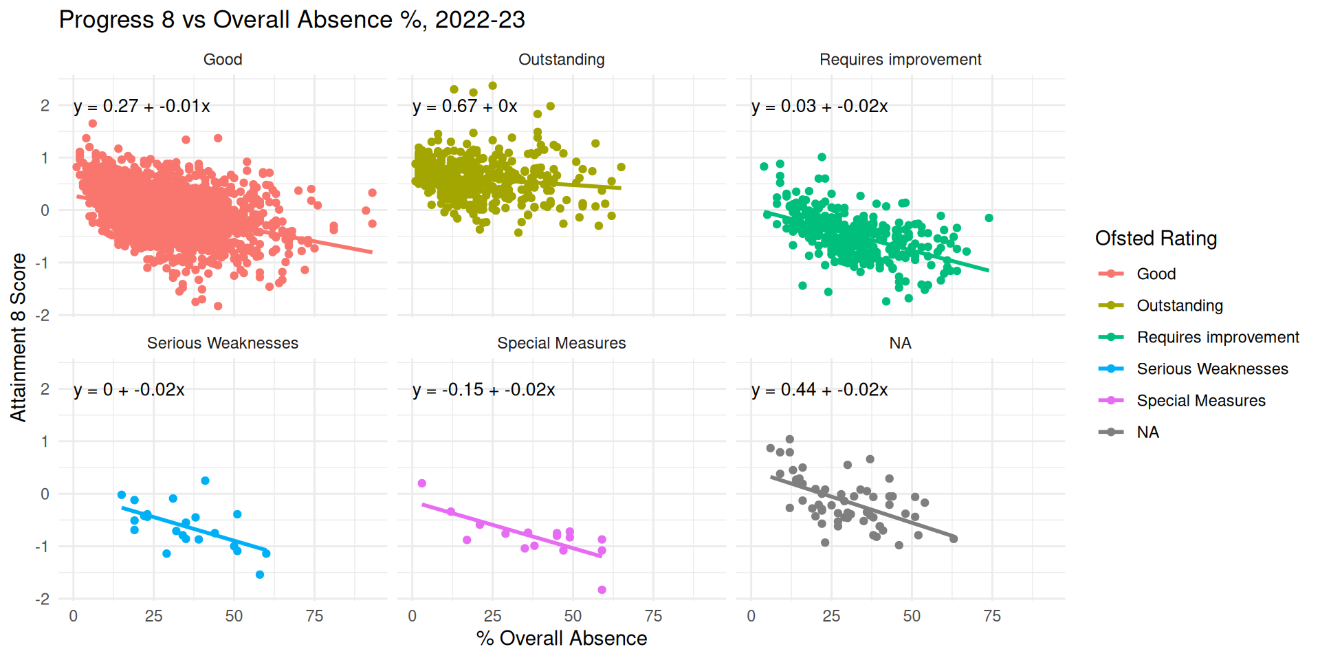
- It’s possible to visualise clusters / sources of non-independence in our model through plotting relationships for different categorical variables
- We are likely to have clustering / non-independence if these plots produce different slopes and intercepts
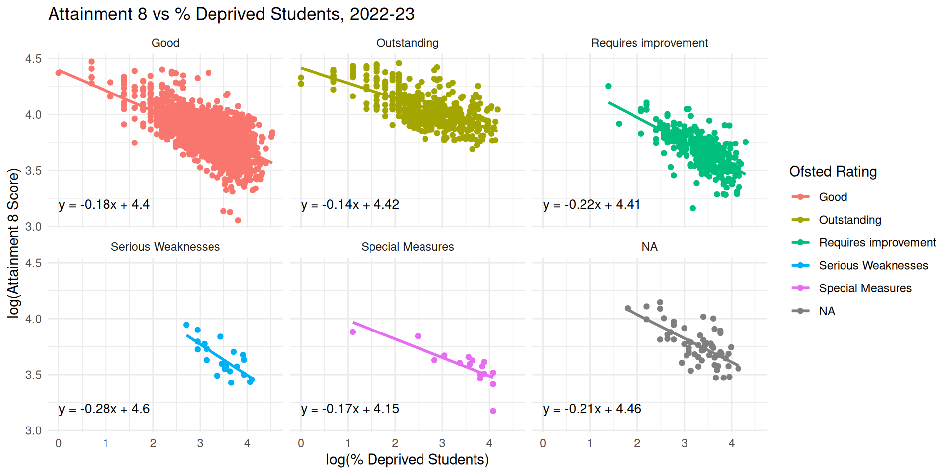
Different Slopes and Intercepts - Attainment 8
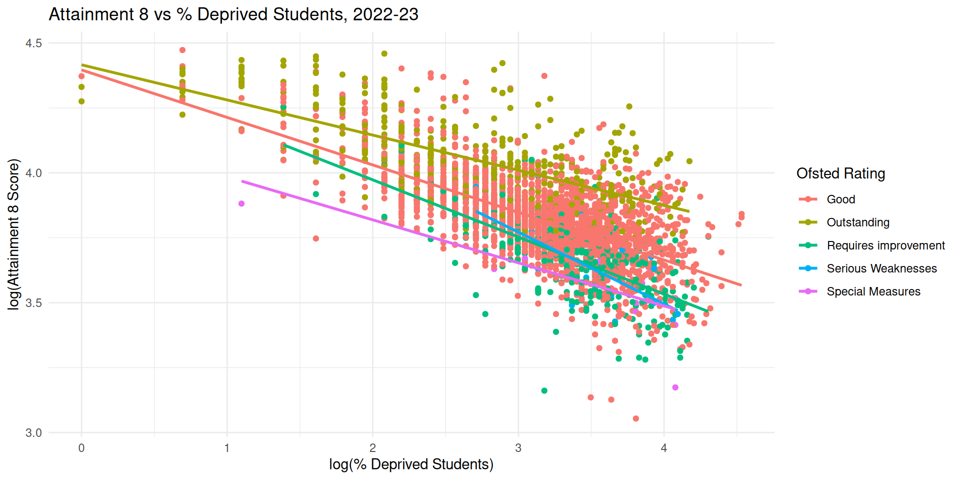
Different Slopes and Intercepts - Attainment 8
Different Slopes and Intercepts - Progress 8
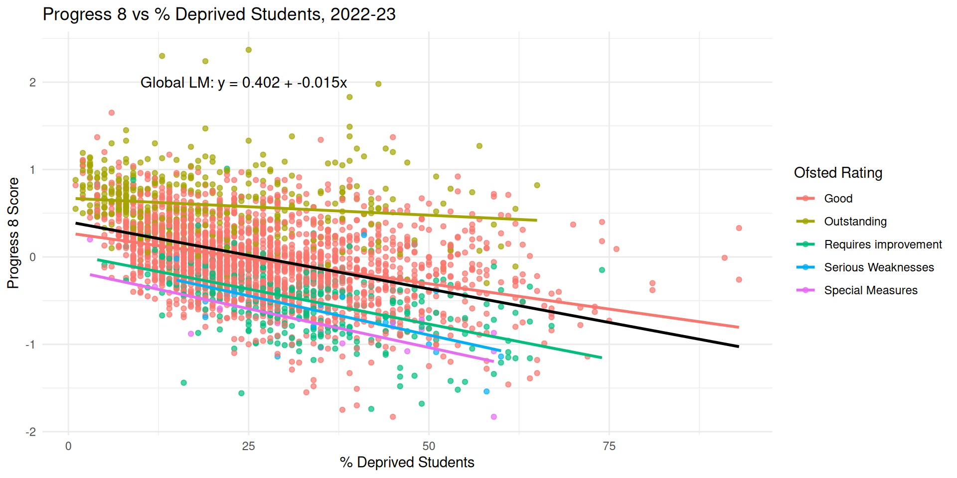
Different Slopes and Intercepts - Progress 8
Different Slopes and Intercepts
- Solution: can we just partition our data and run different models for different groups?
- Answer: Well yes, you could, but we couldn’t then answer questions about:
- whether variation between individual schools (within groups) is more important than between groups (e.g. local authorities or Ofsted ratings)
- how much variation the groups account for themselves
In order to model these grouping factors more explicitly and understand their general impact, we need a new type of model - a linear mixed effects model
Jargon Alert!
- Before we embark on our linear mixed effects journey, there are two key pieces of jargon you need to learn
- Fixed Effects - A Fixed Effect is your traditional explanatory variable (or covariate) whose relationship with the outcome you are primarily interested in estimating for its own sake.
- Example: Proportion of disadvantaged students in a school. You want the single, best-estimated coefficient (\(\beta\)) for this factor.
- Random Effects - A Random Effect is a grouping factor (or nesting factor) whose variability you want to account for, but whose specific individual levels you don’t necessarily want to draw conclusions about.
- Example: The different Ofsted ratings (or individual Schools). You’re interested in how much the relationship varies across these groups, not the specific effect of ‘outstanding’ or ‘Longhill School’
Fixed Effects - More Detail
- Fixed effects estimate the mean relationship across all groups. They represent the “fixed” part of the model that applies to every observation.
- You estimate a single \(\beta\) coefficient for a fixed effect - the population average effect of that variable.
- Fixed effects can be either continuous (e.g., % of disadvantaged students in a school) or categorical (region, Ofsted rating).
- Depending on how you formulate your model, a fixed effect could be a random effect in a different context.
Random Effects - More Detail
- Random effects, (random intercepts and slopes) represent the deviations of each group’s effect from the overall fixed-effect average.
- When you model a grouping factor (like Ofsted Rating) as a random effect, you are not estimating five separate coefficients (one for each rating).
- Instead, you estimate a variance term (\(\sigma^2_{\text{group}}\)) that quantifies how much the true group effects (intercepts and/or slopes) scatter around the overall mean effect.
- Remember: Higher variance = Higher uncertainty, so higher variance groups have less weight in the model
- This allows the model to “borrow strength” across groups to stabilise estimates (the principle of shrinkage).
Random Effects vs Dummy Variables
- Random Effects and Dummy Variables are often exactly the same variable, they are just treated differently in a LME vs OLS model
- In an OLS, the Dummy variable gets a specific coefficient value
- In a LME, the random effect represents the overall variability that that variable brings to the explanation (i.e. how much variability in attainment is down to schools themselves generally, rather than a particular school specifically)
- Where you might have lots of Dummy categories, a random effect might be more suitable
Linear Mixed Effects Models
- A Linear Mixed Effects (LME) model is a more general class of statistical model that features both a fixed-effects component (the population-average parameters) and a random-effects component (the group-specific deviations)
- A common type of LME model is the multilevel model or hierarchical linear model.
- Multilevel models focus specifically on nested data structures, e.g. students in classes \(\rightarrow\) classes within schools \(\rightarrow\) schools within local authorities \(\rightarrow\) local authorities within regions
- All multilevel models are linear mixed effects models, but other types of linear mixed effects models can handle even more types of groupings (e.g. longitudinal - repeated observations over time)
Linear Mixed Effects Models
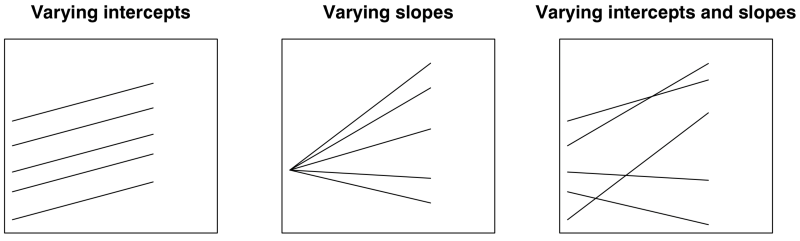
- In practice, LME models essentially result in varying intercepts, slopes or both.
Multilevel Data Structures (Source:Gelman & Hill (2006)) and https://paulrjohnson.net/blog/2022-11-01-multilevel-model-r-cheatsheet/
The Null Model
- The first step in a linear mixed effects model is to fit what is often called a null model (otherwise know as the ‘Variance Components’ / ‘Unconditional Means’ Model)
- Point of the null model is to partition the total variance in the outcome variable (Progress 8 - P8MEA) into the levels or components we think are relevant.
- In our example, we have:
- Schools (Level 1 - our primary unit) and
- Local authority (level 2) - or other grouping factors e.g. Ofsted rating,
- Region (level 3).
- Local authority (level 2) - or other grouping factors e.g. Ofsted rating,
- Schools (Level 1 - our primary unit) and
The Null Model - a 2 Level example
(Intercept)
-0.2646198 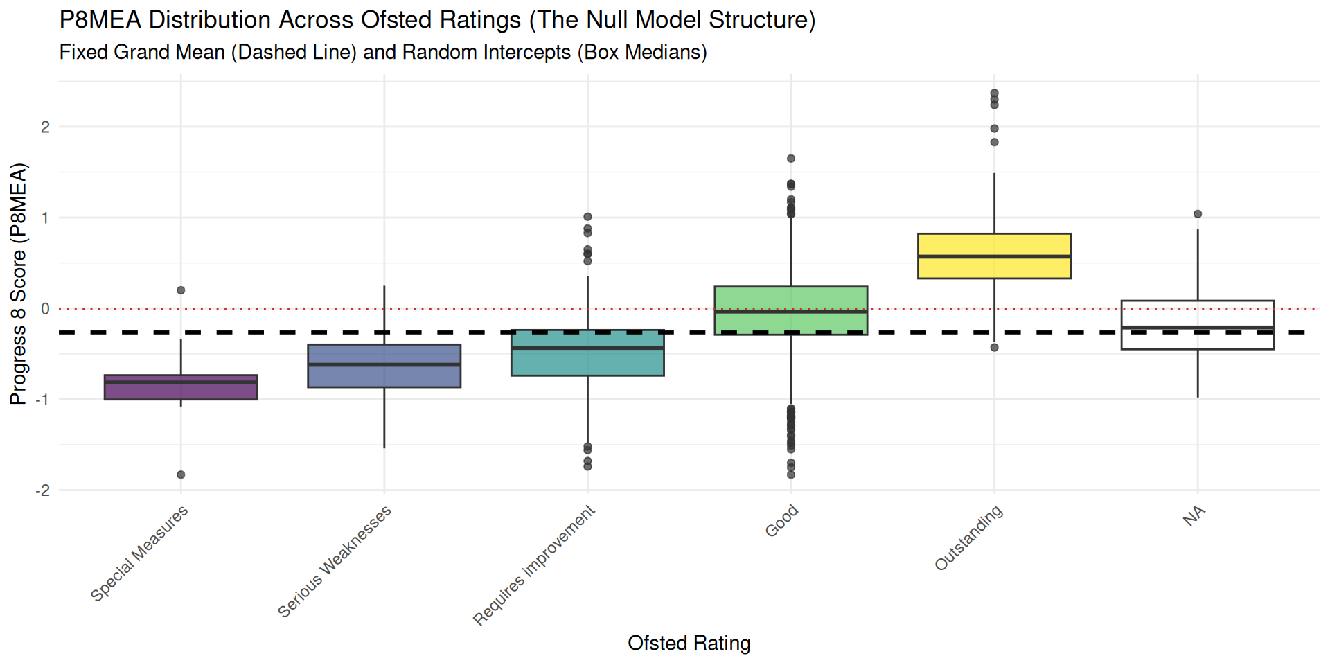
- Most (as box plots hide counts) of the information in the two-level NULL model is contained in this plot!
Shrinkage
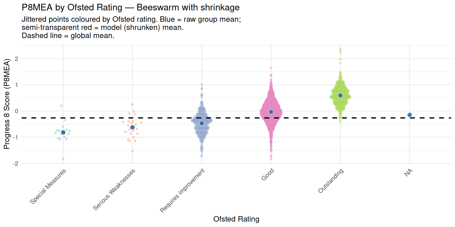
- The global mean in the null model is not just a simple average
- Groups have few observations / high variance / unreliable means are given less importance in the average in a process called shrinkage
- Groups with few observations are ‘shrunk’ towards the overall mean
Shrinkage
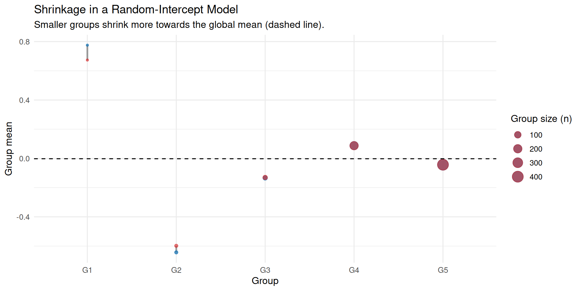
- Shrinkage is another reason why LME models are better than OLS models where clustering exists in the data
- Small groups have less of an influence as their averages get pulled towards the mean - less uncertainty and avoids over-fitting to small groups
The Null Model - a 2 Level example
\[Y_{ij} = \gamma_{00} + u_{0j} + \epsilon_{ij}\] The total variability in outcome \(Y_{ij}\) (Progress 8) for the \(i^{th}\) school in the \(j^{th}\) Ofsted rating is decomposed into:
- Fixed Effect: \(\gamma_{00}\) (gamma - the overall population average - grand/global mean).
- Random Effect - Level 1: \(\epsilon_{ij}\) - Within-Group Variance - the height of each individual box and the length of its whiskers. Taller boxes and longer whiskers indicate more variability among schools within that single rating category.
- Random Effect - Level 2: \(u_{0j}\) - Between-Group Variance
Level 1 - Within-Group Variance
\[ Y_{ij} = \beta_{0j} + \epsilon_{ij} \]
- The Progress 8 Outcome: \(Y_{ij}\)
- The within-group intercept: \(\beta_{0j}\) for the specific Ofsted rating \(j\). This represents the true mean Progress 8 for all schools within that rating.
- The Level 1 residual error: \(\epsilon_{ij}\) (or “school-level error”). This is the deviation of the \(i^{th}\) school’s P8MEA from its own Ofsted group’s mean (\(\beta_{0j}\)).
- Assumption: \(\epsilon_{ij} \sim N(0, \sigma^2_{\epsilon})\) where \(\sigma^2_{\epsilon}\)
Level 1 - Within-Group Variance
\[\epsilon_{ij} \sim N(0, \sigma^2_{\epsilon})\]
| Notation | Meaning |
| \(\epsilon_{ij}\) | The Level 1 Residual Error (or “within-group error”) for the \(i\)-th school in the \(j\)-th Ofsted rating. |
| \(\sim\) | “Is distributed as” or “Follows the distribution.” |
| \(N(\dots)\) | The Normal (Gaussian) Distribution. |
| \(0\) | The Mean of the distribution = 0. |
| \(\sigma^2_{\epsilon}\) | The Within-Group Variance of the the error term. Sigma - \(\sigma\) is commonly used to represent standard deviation. Variance is \(\sigma^2\) |
Level 2 - Between-Group Variance
\[ \beta_{0j} = \gamma_{00} + u_{0j} \]
- Level 1 intercept \(\beta_{0j}\): The mean Progress 8 for the \(j^{th}\) Ofsted rating
- The grand mean \(\gamma_{00}\): the overall fixed intercept. This is the mean Progress 8 averaged across all Ofsted ratings. The dotted black line on our earlier plot
- Level 2 residual error \(u_{0j}\): “group-level error”. This is the deviation of the \(j^{th}\) Ofsted rating’s mean (\(\beta_{0j}\)) from the grand mean (\(\gamma_{00}\)).
- Assumption: \(u_{0j} \sim N(0, \sigma^2_{u_{0}})\) where \(\sigma^2_{u_{0}}\) is the Between-Group Variance (or Level 2 variance/Random Intercept Variance).
Total Variance
- Between-Group Variance (\(\sigma^2_{\text{Between}}\) - or more generally \(\sigma^2_{u_{0}}\)): The variability in average P8MEA that exists between the different Ofsted ratings.
- Within-Group (Residual) Variance (\(\sigma^2_{\text{Within}}\) - or more generally \(\sigma^2_{\epsilon}\)): The variability in P8MEA that exists between schools within each rating (i.e., the school-level differences).
- Total Variance is simply the sum of these two
\[\sigma^2_{\text{Total}} = \sigma^2_{\text{Between}} + \sigma^2_{\text{Within}}\] \[\sigma^2_{\text{Total}} = \sigma^2_{u_{0}} + \sigma^2_{\epsilon}\]
The Intraclass Correlation Coefficient (ICC)
\[\text{ICC} = \frac{\text{Between-Group Variance}}{\text{Total Variance}} = \frac{\sigma^2_{u_{0}}}{\sigma^2_{u_{0}} + \sigma^2_{\epsilon}}\]
- This ICC is simply the ratio between the between the between group variance and the total variance
- The higher the ICC (closer to 1), the more variance is due to differences between groups (i.e. differences between the Ofsted rating of schools) than within groups (i.e. between schools within Ofsted rating bands)
- A high ICC is a strong indication that a multilevel model is a suitable modelling strategy to pursue to try and explain these group-level differences
Visualising The ICC
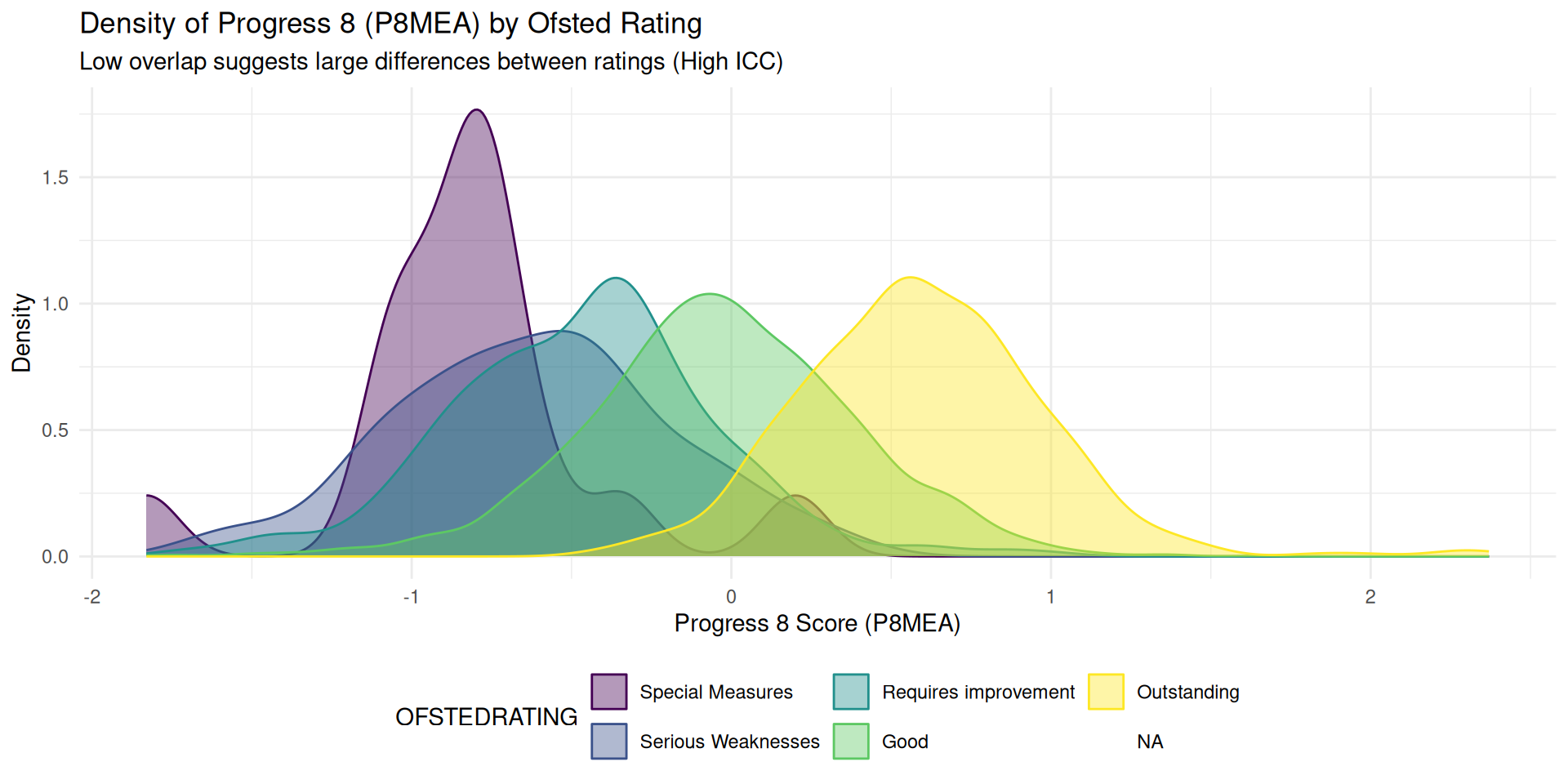
- High ICC = distinct, non-overlapping humps
- Low ICC = density plots all overlapping on-top of each other
The Null Model - Fixed Global Intercept & Fixed Random Effect Slopes
- Using Paul Johnson’s excellent guide for syntax, the null model in R follows this format:
y ~ 1 + (1 | g) - Fixed effects outside of the brackets. The first
1just tells the model to use a fixed global intercept (global averagey) - Random Effects are inside the brackets
(...|...)- To the left of the pipe symbol
|we have a1as all slopes are fixed as groupgaverage ofy - To the right of the vertical bar or pipe symbol
|we have the grouping variablegitself.
- To the left of the pipe symbol
- The full model in R would like like:
lme_model1 <- lmer(P8MEA ~ 1 + (1|OFSTEDRATING), data = ...)
Running The Null Model
Linear mixed model fit by REML ['lmerMod']
Formula: P8MEA ~ 1 + (1 | OFSTEDRATING)
   Data: england_filtered_clean

REML criterion at convergence: 3156.8

Scaled residuals:
    Min      1Q  Median      3Q     Max
-4.3316 -0.6163  0.0060  0.6152  4.2823

Random effects:
 Groups       Name        Variance Std.Dev.
 OFSTEDRATING (Intercept) 0.3146   0.5609
 Residual                 0.1718   0.4145
Number of obs: 2906, groups:  OFSTEDRATING, 5

Fixed effects:
            Estimate Std. Error t value
(Intercept) -0.2646 0.2523 -1.049- Fixed Effect: Global Average
y(Progress 8) is -0.26 - Random Effect: Progress 8 varies by 0.31 points on average between Ofsted categories
- Residual variation between schools within categories is smaller: 0.17 points
The NULL model ICC
# ICC by Group

Group        |   ICC
--------------------
OFSTEDRATING | 0.647- ICC of 0.647 means around 65% of the total variation in Progress 8 scores is explained by differences between OFSTED rating groups
- The remaining 35% is due to variation within those groups (i.e. between individual schools)
- ICC of 65% is very high - Schools in the same OFSTED category tend to have very similar Progress 8 scores
- High ICC means clustering is important. Ignoring it (e.g., using OLS) would underestimate uncertainty - justifies using a LME model
NULL Model Visualisation
Model with a Fixed Effect Predictor
y ~ x + (1 | g)- In this model, each group in the Random Effect part of the model has it’s own intercept but a fixed slope still -
(1 | g) - Adding a variable into the Fixed Effect part of the model shows how
xinfluencesyacross all groups - The Null Model asks: “How much do groups differ, ignoring everything else?”
- This model asks: “How does
xaffecty, while still accounting for group differences?”
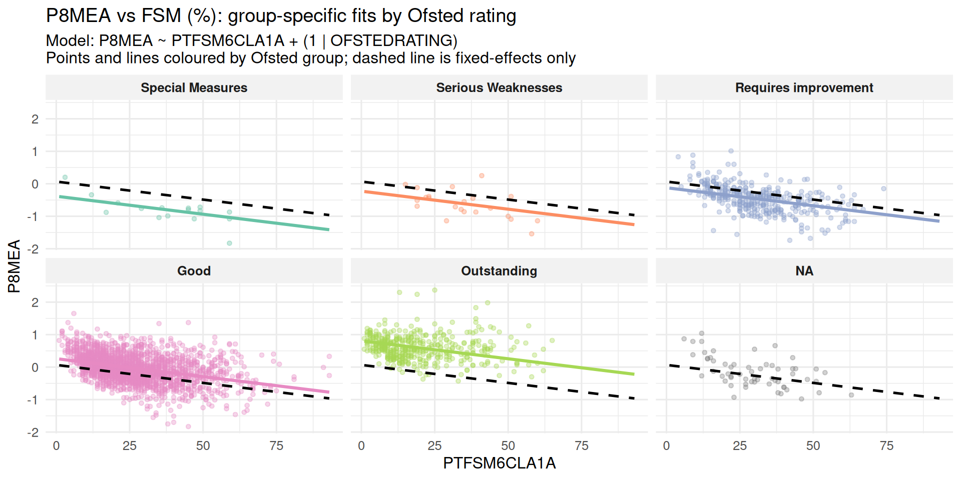
Model with a Fixed Effect Predictor
Model with a Fixed Effect Predictor
Linear mixed model fit by REML ['lmerMod']
Formula: P8MEA ~ PTFSM6CLA1A + (1 | OFSTEDRATING)
   Data: england_filtered_clean

REML criterion at convergence: 2744

Scaled residuals:
    Min      1Q  Median      3Q     Max
-4.1283 -0.6451 -0.0364  0.5935  4.7671

Random effects:
 Groups       Name        Variance Std.Dev.
 OFSTEDRATING (Intercept) 0.2320   0.4817
 Residual                 0.1485   0.3853
Number of obs: 2906, groups:  OFSTEDRATING, 5

Fixed effects:
              Estimate Std. Error t value
(Intercept)  0.0673133  0.2174828    0.31
PTFSM6CLA1A -0.0110830  0.0005174  -21.42

Correlation of Fixed Effects:
            (Intr)
PTFSM6CLA1A -0.071- Adding the fixed effect variable reduces Random Effect Ofsted group variance from 0.31 to 0.23. Some between group variance now captured by PTFSM6CLA1A
- Fixed effect of % disadvantaged students highly significant
- REML criterion: 3156.8 → 2729.2 indicating better fit
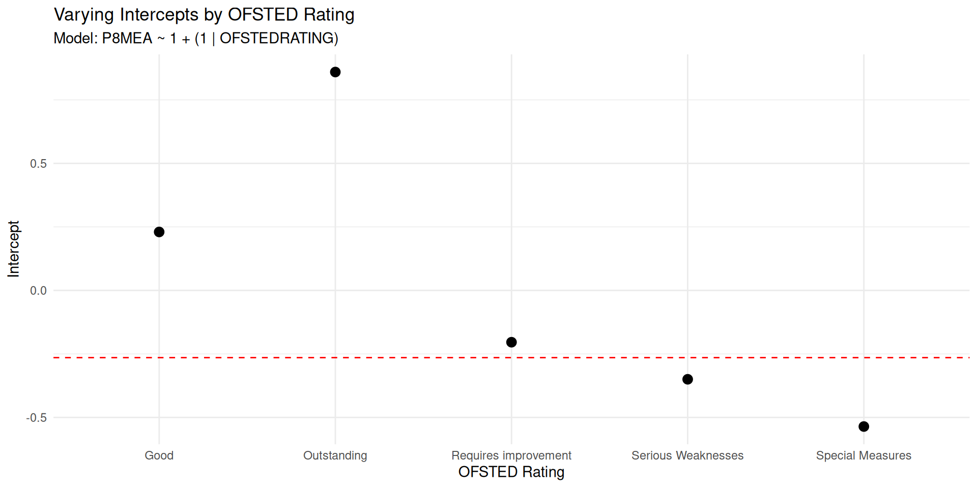
Model with a Fixed Effect Predictor
                     (Intercept)
Special Measures      -0.5358379
Serious Weaknesses    -0.3498755
Requires improvement  -0.2039681
Good                   0.2300834
Outstanding 0.8595982- While the main summary doesn’t show the specific intercepts for each group, these can be extracted from the model object using the
ranef(random effect) function in R - These Random Effect intercepts are the deviation from the global mean and effectively show what is on the plot when combined with the Fixed Effect parameter
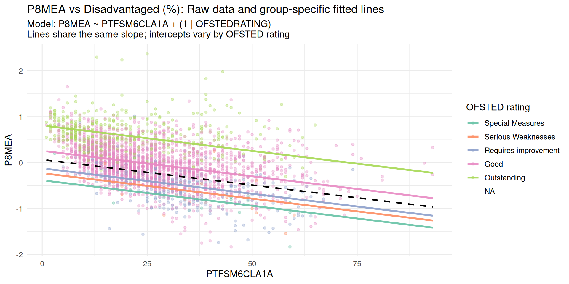
Model with a Fixed Effect Predictor
Random Intercept and Random Slope Model
- Right back at the beginning of the lecture when we plotted each Ofsted Subset as a separate regression model, it was clear that the relationship between % Disadvantaged Pupils in a school & Progress 8 had different slopes as well as intercepts
y ~ x + (x | g)- Adding the random slopes simply requires the predictor variable to the left of the pipe in the Random effects bracket
(x | g) - In this model each group has its own baseline (intercept) and its own relationship between
xandy(whereas in the last model the relationship betweenxandywas assumed constant across groups)
Random Intercept and Random Slope Model
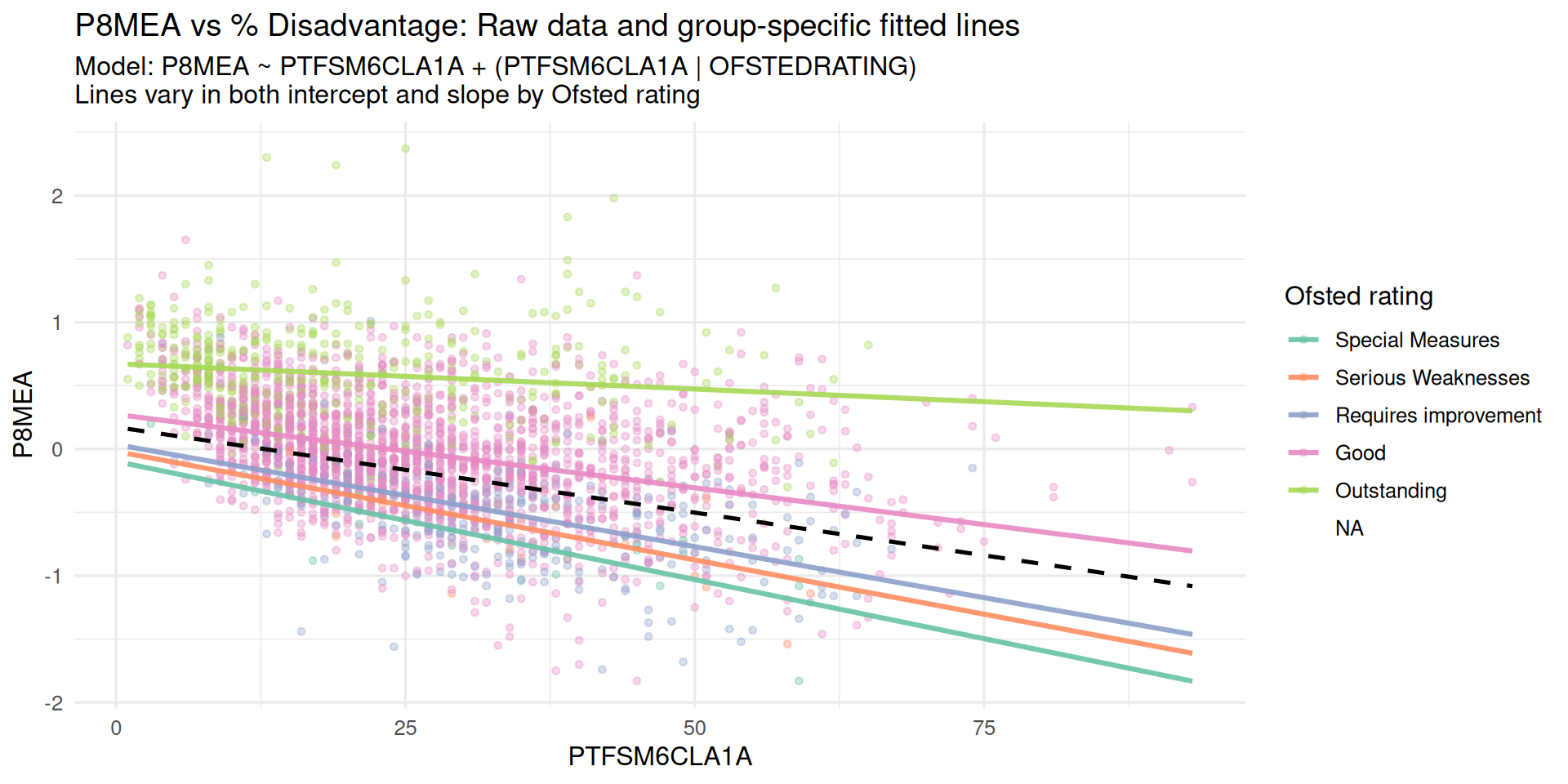
- Most Ofsted Groups are similar to the mean
- Although for Outstanding schools, the proportions of disadvantage appear to have very little effect on Progress 8
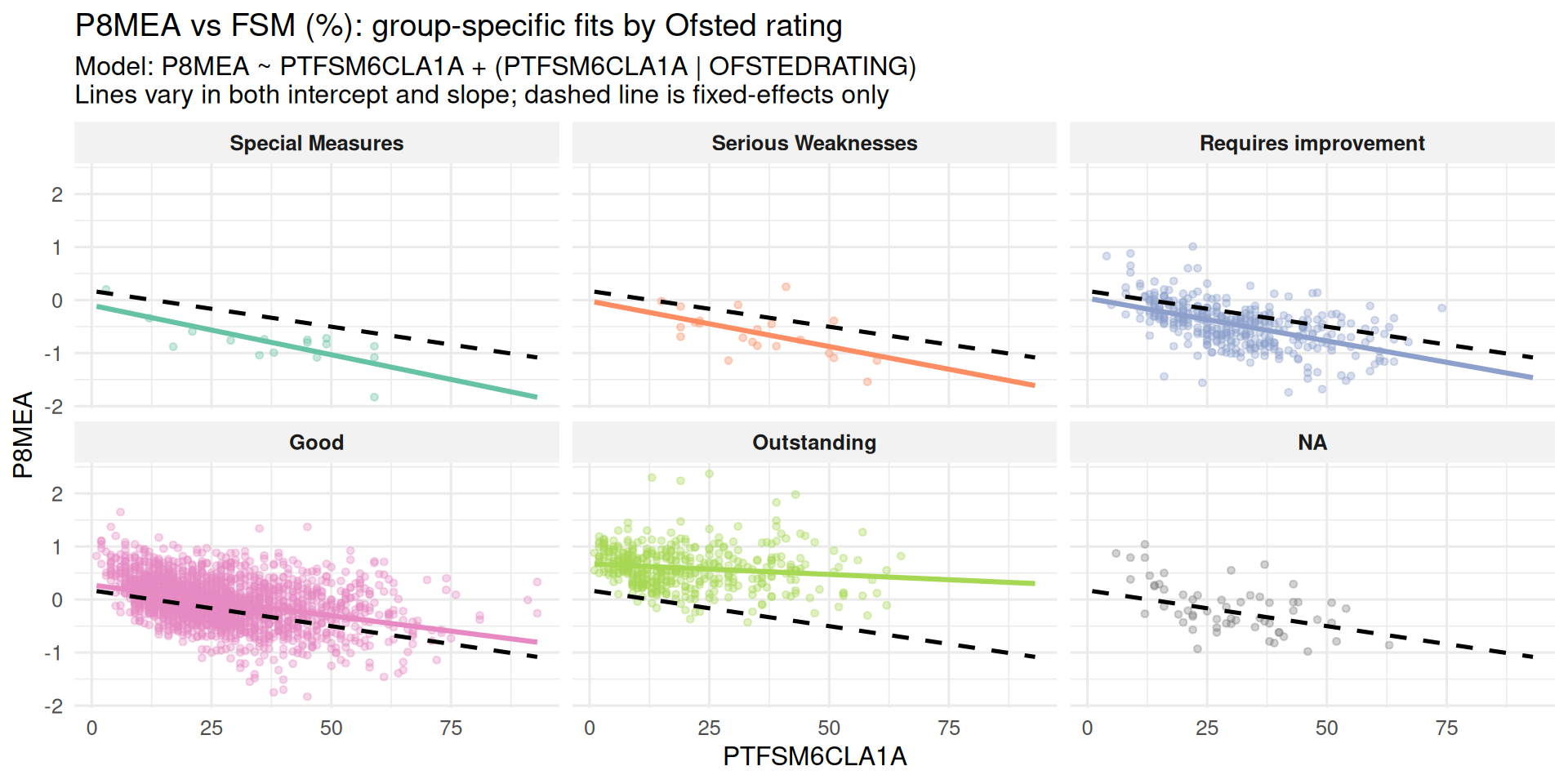
Random Intercept and Random Slope Model
Linear mixed model fit by REML ['lmerMod']
Formula: P8MEA ~ PTFSM6CLA1A + (PTFSM6CLA1A | OFSTEDRATING)
   Data: england_filtered_clean

REML criterion at convergence: 2702.1

Scaled residuals:
    Min      1Q  Median      3Q     Max
-4.1370 -0.6525 -0.0411  0.5920  4.6984

Random effects:
 Groups       Name        Variance  Std.Dev. Corr
 OFSTEDRATING (Intercept) 9.851e-02 0.313870
              PTFSM6CLA1A 3.549e-05 0.005957 1.00
 Residual                 1.463e-01 0.382504
Number of obs: 2906, groups:  OFSTEDRATING, 5

Fixed effects:
             Estimate Std. Error t value
(Intercept)  0.172412   0.142010   1.214
PTFSM6CLA1A -0.013490   0.002723  -4.954

Correlation of Fixed Effects:
            (Intr)
PTFSM6CLA1A 0.959
optimizer (nloptwrap) convergence code: 0 (OK)
boundary (singular) fit: see help('isSingular')- REML dropped from 2744 → 2702, meaning the second model fits slightly better (lower REML = better fit)
- However, slope variance 3.549e-05 (0.000035) very small (i.e. possibly not worth additional complexity compared to fixed slope model)
- And correlation of 1.0 between slope and intercept in Random effects is problematic
- Suggests visual difference in Outstanding Ofsted not statistically reliable.
Random Intercept and Random Slope Model
# Extract random effects for each OFSTED group
ranef_values <- ranef(lme3)$OFSTEDRATING

# Fixed slope
fixed_slope <- fixef(lme3)["PTFSM6CLA1A"]

# Add random deviations to get group-specific slopes
group_slopes <- fixed_slope + ranef_values$PTFSM6CLA1A

# Combine into a tidy data frame
slopes_df <- data.frame(
  OFSTEDRATING = rownames(ranef_values),
  slope = group_slopes
)

print(slopes_df)
OFSTEDRATING slope
1 Special Measures -0.018639324
2 Serious Weaknesses -0.017126695
3 Requires improvement -0.016104820
4 Good -0.011586886
5 Outstanding -0.003994586- Again, while the standard model outputs don’t print the slope parameters, these can be extracted
Random Intercept and Random Slope Model
Other Linear Mixed Effects Models
| Element | Meaning | Sample Equation |
|---|---|---|
(1|g) |
Null Model or Varying Intercept Model | P8 ~ 1 + (1 | OFSTEDRATING) |
(1|g1/g2) |
Multilevel Model with intercept varying within g1 and for g2 within g1 | P8 ~ 1 + (1 | LocalAuthority/Region) |
(1|g1) + (1|g2) |
Intercept varying among g1 and g2 | P8 ~ 1 + (1 | OFSTEDRATING) + (1 | Region) |
(0+x|g) |
Varying Slope Model | P8 ~ Disadvantage + (0 + Disadvantage | OFSTEDRATING) |
x + (x|g) |
Varying and correlated intercepts and slopes | P8 ~ Disadvantage + (Disadvantage | OFSTEDRATING) |
x + (x||g) |
Uncorrelated Intercepts and Slopes | P8 ~ Disadvantage + (Disadvantage || OFSTEDRATING) |
Last Week’s Attainment 8 Best Model
Call:
lm(formula = log(ATT8SCR) ~ log(PTFSM6CLA1A) + log(PERCTOT) +
    log(PNUMEAL) + OFSTEDRATING + gor_name + PTPRIORLO + ADMPOL_PT,
    data = england_filtered_clean, na.action = na.exclude)

Residuals:
     Min       1Q   Median       3Q      Max
-0.37723 -0.04528  0.00333  0.04912  0.30081

Coefficients:
                                   Estimate Std. Error t value Pr(>|t|)
(Intercept)                       4.5966533  0.0178852 257.009  < 2e-16 ***
log(PTFSM6CLA1A)                 -0.0699264  0.0036900 -18.950  < 2e-16 ***
log(PERCTOT)                     -0.2244960  0.0074455 -30.152  < 2e-16 ***
log(PNUMEAL)                      0.0179676  0.0016174  11.109  < 2e-16 ***
OFSTEDRATING.L                    0.1141381  0.0134587   8.481  < 2e-16 ***
OFSTEDRATING.Q                    0.0223425  0.0113333   1.971 0.048773 *
OFSTEDRATING.C                    0.0094244  0.0118583   0.795 0.426824
OFSTEDRATING^4                   -0.0130171  0.0085375  -1.525 0.127442
gor_nameEast of England           0.0056999  0.0063522   0.897 0.369630
gor_nameLondon                    0.0266978  0.0065474   4.078 4.67e-05 ***
gor_nameNorth East                0.0202813  0.0084342   2.405 0.016250 *
gor_nameNorth West               -0.0139159  0.0060835  -2.287 0.022239 *
gor_nameSouth East               -0.0128394  0.0060587  -2.119 0.034161 *
gor_nameSouth West                0.0254495  0.0065872   3.863 0.000114 ***
gor_nameWest Midlands             0.0058630  0.0063008   0.931 0.352183
gor_nameYorkshire and the Humber  0.0199996  0.0065661   3.046 0.002341 **
PTPRIORLO                        -0.0069371  0.0002201 -31.525  < 2e-16 ***
ADMPOL_PTOTHER NON SEL            0.0154098  0.0060930   2.529 0.011488 *
ADMPOL_PTSEL                      0.0806871  0.0098281   8.210 3.30e-16 ***
---
Signif. codes:  0 '***' 0.001 '**' 0.01 '*' 0.05 '.' 0.1 ' ' 1

Residual standard error: 0.07492 on 2883 degrees of freedom
  (59 observations deleted due to missingness)
Multiple R-squared:  0.8443,    Adjusted R-squared:  0.8433
F-statistic: 868.5 on 18 and 2883 DF,  p-value: < 2.2e-16
A Linear Mixed Effects Revision
“He threw everything but the kitchen sink at it!”
- Not quite everything, but:
- Fixed Effects: % Disadvantaged Students, % pupils where English not first language, % Overall Absence, % of pupils at the end of key stage 4 with low prior attainment at the end of key stage 2, Admissions Policy
- Random Effects: Ofsted Rating and nested (multilevel) Local Authority and Regional Geographic effects
My Final kitchen sink model!!
Linear mixed model fit by REML ['lmerMod']
Formula: log(ATT8SCR) ~ log(PTFSM6CLA1A) + log(PERCTOT) + log(PNUMEAL) +
    PTPRIORLO + ADMPOL_PT + (1 | OFSTEDRATING) + (1 | gor_name/LANAME)
   Data: england_filtered_clean

REML criterion at convergence: -6867.1

Scaled residuals:
    Min      1Q  Median      3Q     Max
-5.7645 -0.5790  0.0301  0.6358  4.5633

Random effects:
 Groups          Name        Variance  Std.Dev.
 LANAME:gor_name (Intercept) 0.0006878 0.02623
 gor_name        (Intercept) 0.0002478 0.01574
 OFSTEDRATING    (Intercept) 0.0032801 0.05727
 Residual                    0.0050031 0.07073
Number of obs: 2902, groups:
LANAME:gor_name, 151; gor_name, 9; OFSTEDRATING, 5

Fixed effects:
                         Estimate Std. Error t value
(Intercept)             4.6350167  0.0320063 144.816
log(PTFSM6CLA1A)       -0.0753777  0.0039754 -18.961
log(PERCTOT)           -0.2237835  0.0073213 -30.566
log(PNUMEAL)            0.0143445  0.0017594   8.153
PTPRIORLO              -0.0068604  0.0002199 -31.202
ADMPOL_PTOTHER NON SEL  0.0059090  0.0089869   0.658
ADMPOL_PTSEL            0.0748478  0.0097318   7.691

Correlation of Fixed Effects:
            (Intr) l(PTFS l(PERC l(PNUM PTPRIO ADMPNS
l(PTFSM6CLA -0.106
lg(PERCTOT) -0.377 -0.354
lg(PNUMEAL) -0.080 -0.257  0.165
PTPRIORLO    0.110 -0.412 -0.208 -0.150
ADMPOL_PTNS -0.265 -0.044  0.016 -0.013  0.074
ADMPOL_PTSE -0.254  0.180  0.015 -0.215  0.286  0.554
My Final kitchen sink model!!
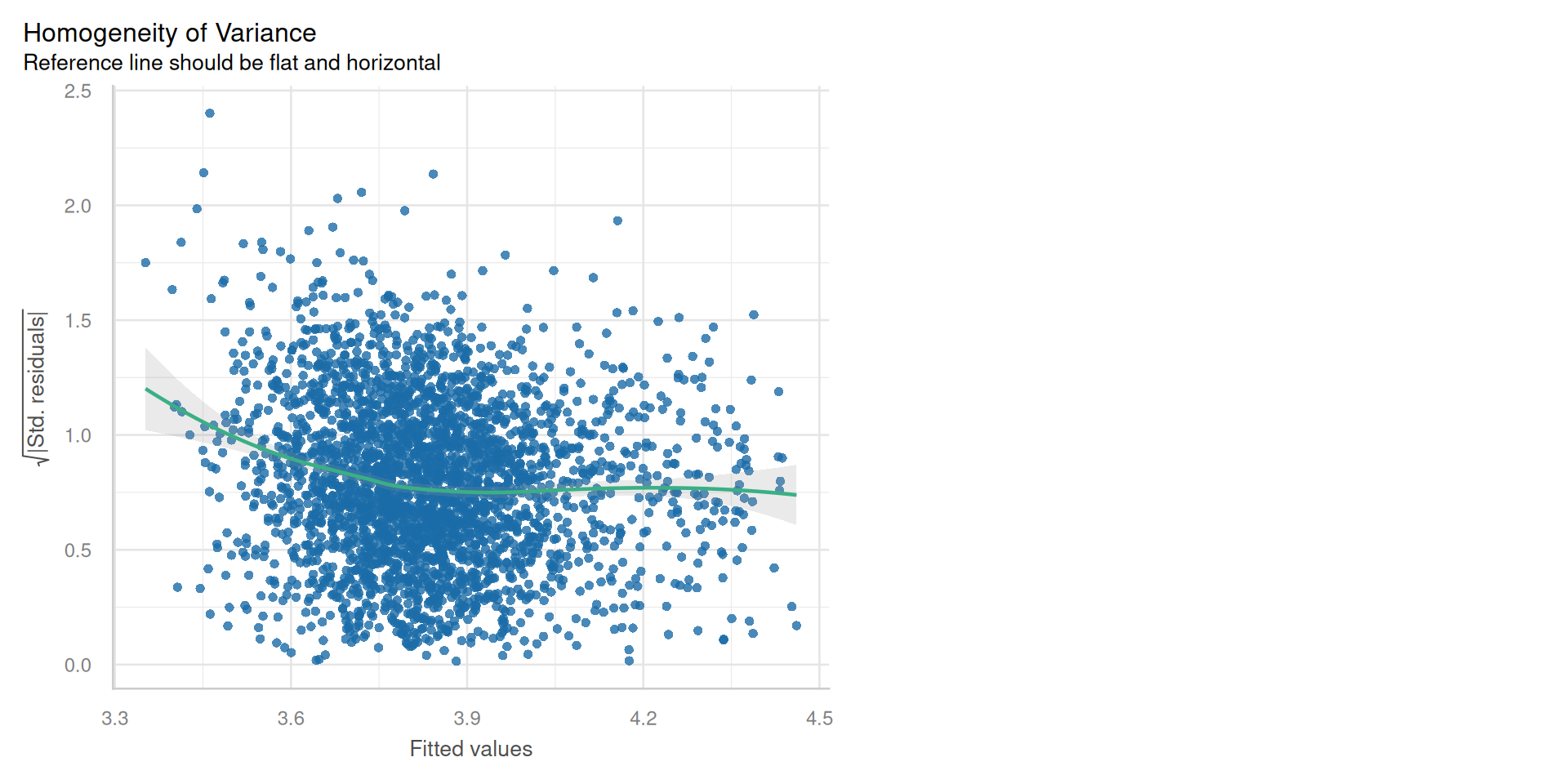
My Final kitchen sink model!!
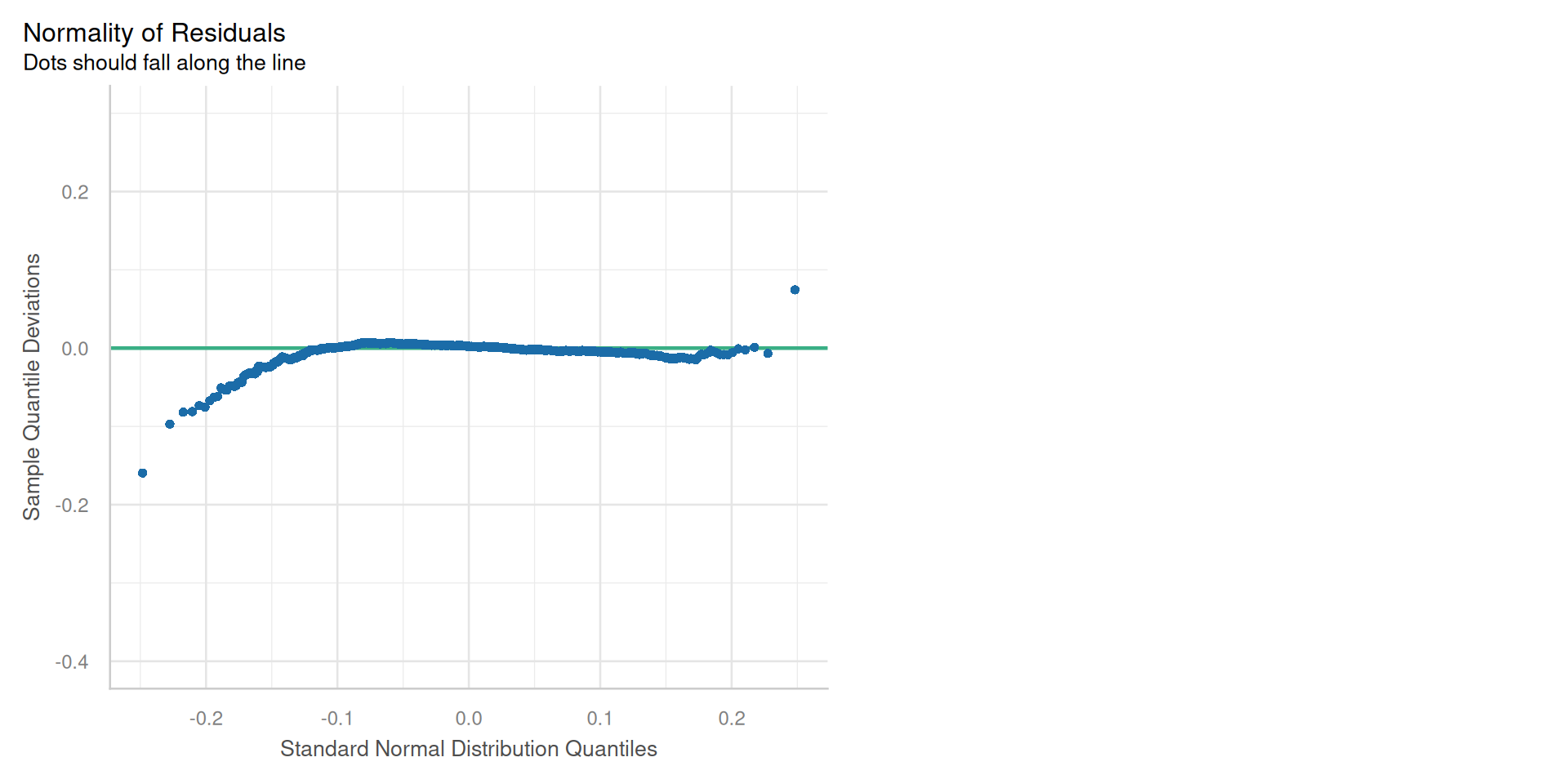
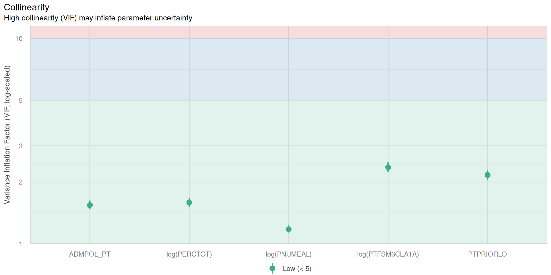
My Final kitchen sink model!!
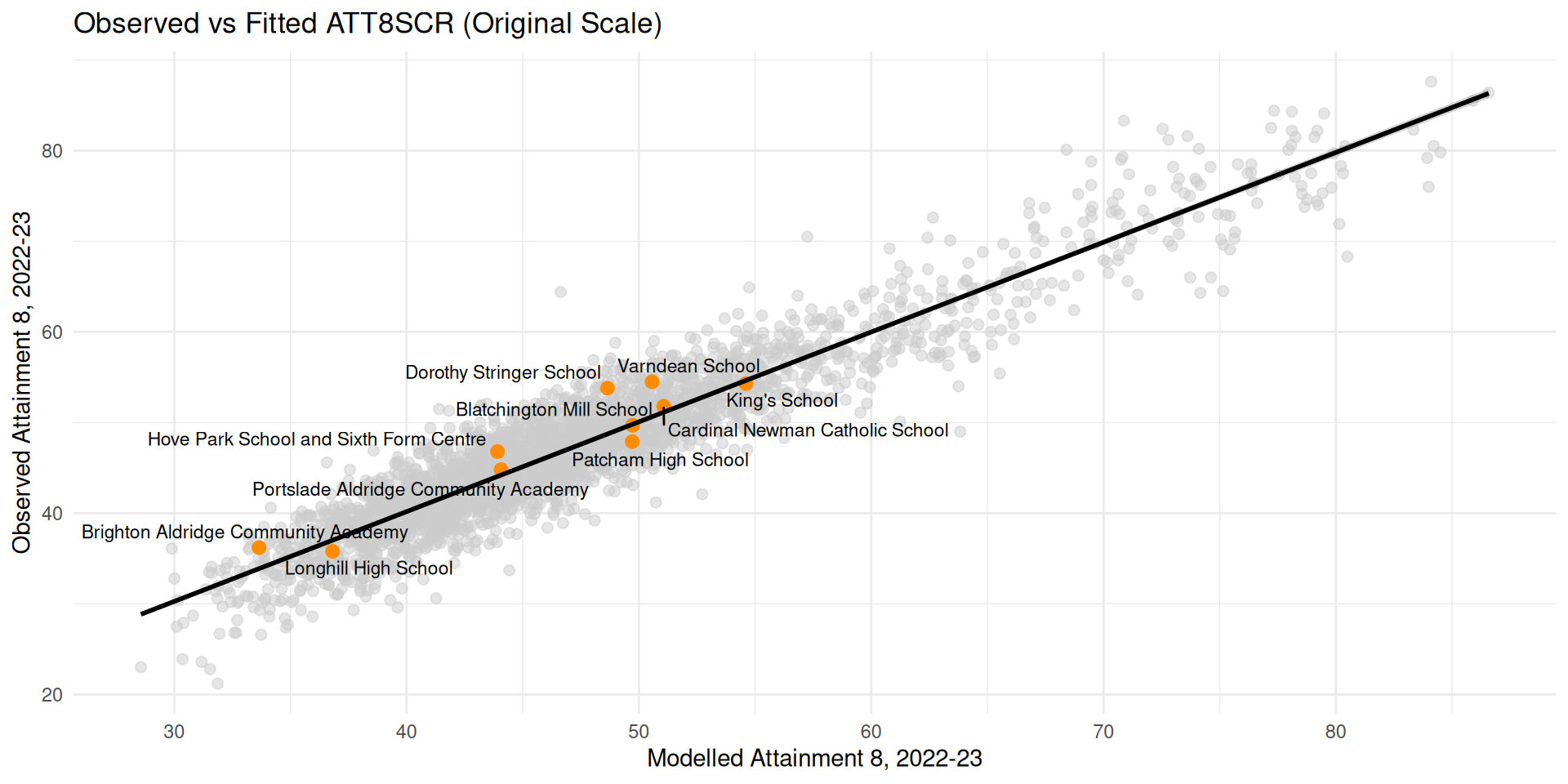
- Very good fit, \(R^2\) = 86%
Interpreting the Final Model - Random Effects
| Group | Variance | Std. Dev |
|---|---|---|
| Intercept Local Authority Within Region | 0.00069 | 0.026 |
| Intercept Region | 0.00025 | 0.016 |
| Intercept OFSTEDRATING | 0.00328 | 0.057 |
| Residual School-to-School | 0.00500 | 0.071 |
- Random effects represent variation across levels (categories) within a grouping factor
- Larger variance = more difference between those levels (e.g. London to SE in Region)
- SD (sqrt(variance)) is typical size of deviation from the overall mean for a group.
- A typical OFSTED level differs from the overall mean by about ±1 SD (≈ 0.057 on the log scale)
- \(exp(\sigma^2_{\text{OFSTEDRATING}})-1 ≈ exp(0.0573)−1 ≈ 0.059 ≈ 5.9\%\)
- Baseline Attainment 8 (from null model) - \(exp(3.75644) = 42.8\)
- Average jump between Ofsted Rating Groups worth \(42.8 \times 0.059 ≈ 2.52\) GCSE points
Interpreting the Final Model - Random Effects
| Group | Variance | Std. Dev |
|---|---|---|
| Intercept Local Authority Within Region | 0.00069 | 0.026 |
| Intercept Region | 0.00025 | 0.016 |
| Intercept OFSTEDRATING | 0.00328 | 0.057 |
| Residual School-to-School | 0.00500 | 0.071 |
- Residual variance (0.0050) represents the within-group variation—differences between individual schools after accounting for fixed effects and the random intercepts for OFSTED, LA, and region
- Since 0.0050 (residual) > 0.00328 (OFSTED) and much larger than LA or region variances, most of the unexplained variation is within groups (school-to-school differences) rather than between OFSTED categories or geographic clusters.
Interpreting the Final Model - Random Effects
What about specific point differences between Ofsted Groups?
                     (Intercept)
Special Measures     -0.06084082
Serious Weaknesses   -0.03189554
Requires improvement -0.01942173
Good                  0.03077845
Outstanding 0.08137964- Good vs Requires Improvement: \(\Delta\log = 0.0308−(−0.0194) = 0.0502\)
- Good vs RI: \(exp(0.0502) ≈ 1.0515 → +5.15\%\)
- Good vs RI: \(42.8 \times ≈ 0.0515 ≈ 2.2\) GCSE Points
Interpreting the Final Model - Random Effects
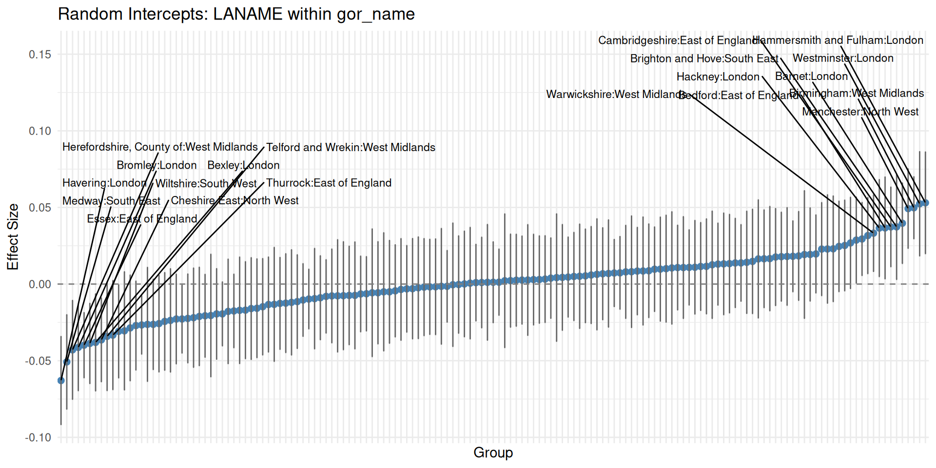
- Extracting the random effects and their variances for individual groups and plotting them in a caterpillar plot allows you to see which groups are meaningfully different from the average
- If a group’s confidence interval doesn’t cross the 0 line, it’s an interesting case (oh look, there’s Brighton!)
- Similar to looking for significant dummies in an OLS model - although these are shrunken estimates
Interpreting the Final Model - Fixed Effects
Fixed Effects
| OLS | LMM | |
|---|---|---|
| (Intercept) | 4.597 (0.023)*** | 4.635 (0.032)*** |
| log(PTFSM6CLA1A) | -0.070 (0.004)*** | -0.075 (0.004)*** |
| log(PERCTOT) | -0.224 (0.010)*** | -0.224 (0.007)*** |
| log(PNUMEAL) | 0.018 (0.002)*** | 0.014 (0.002)*** |
| PTPRIORLO | -0.007 (0.000)*** | -0.007 (0.000)*** |
| ADMPOL_PTOTHER NON SEL | 0.015 (0.006)* | 0.006 (0.009) |
| ADMPOL_PTSEL | 0.081 (0.010)*** | 0.075 (0.010)*** |
| R2 (Conditional) | 0.843 | 0.856 |
- Very little change in the fixed effects from the original OLS model
- Only the very small ‘other non selective school’ group loses significance
- Most coefficients and the overall intercept very similar
Interpreting the Final Model - Fixed Effects
| Predictor | Scenario | Log shift = equation for % change | % change | Raw points = 42.8 baseline x % change |
|---|---|---|---|---|
| % Overall Absence - log(PERCTOT) | 40% → 30% | −0.2238 × log(30/40) | +6.65% | +2.85 |
| 20% → 10% | −0.2238 × log(10/20) | +16.78% | +7.18 | |
| % Disadvantage - log(PTFSM6CLA1A) | 40% → 30% | −0.0754 × log(30/40) | +2.19% | +0.94 |
| 20% → 10% | −0.0754 × log(10/20) | +5.36% | +2.30 | |
| Prior low attainment - (PTPRIORLO) | 40 → 30 pp | −0.00686 × (−10) | +7.10% | +3.04 |
| 20 → 10 pp | −0.00686 × (−10) | +7.10% | +3.04 |
- Note - final column only illustrative as using global average
Wrapping it all up
- In our final model we are to see that controlling for:
- absence, disadvantage, prior attainment, selectivity in admissions and English not as a first language while also controlling for the variability within and between geographical locations and Ofsted ratings, Prior Low Attainment at KS2 is the most important predictor of Attainment 8
- The effects of prior low attainment are linear, but the effects of absence and disadvantage are felt more strongly where low levels change and less strongly where higher levels change
- Reducing absence is significantly more likely to improve Attainment 8 than reducing levels of disadvantage in a school
- In terms of random effects, while not causal a jump between Ofsted ratings is worth, on average, about 2.5 GSCE points - similar to a reduction in disadvanage in a school from 20%-10%.
Back to our Week 6 Reserarch Question(s)
- What are the factors that affect school-level educational attainment in Brighton and Hove?
- To what extent is attainment driven by social mixing?
- Are there any other factors that are relevant?
- What are the implications of this for local policy?
- Can regression help us and, if it can, how can we go about carefully building a regression model to help us answer these questions?
Custom Policy - Brighton Schools
| Variable | Brighton Aldridge Community Academy | Longhill High School | Patcham High School |
|---|---|---|---|
| PERCTOT | 16.2 | 13.4 | 9.2 |
| PTFSM6CLA1A | 45.0 | 29.0 | 19.0 |
| PNUMEAL | 12.3 | 7.9 | 6.4 |
| PTPRIORLO | 37.0 | 34.0 | 14.0 |
| ADMPOL_PT | OTHER NON SEL | OTHER NON SEL | OTHER NON SEL |
| RE: OFSTEDRATING | -0.019 | -0.019 | 0.031 |
| RE: gor_name | -0.015 | -0.015 | -0.015 |
| RE: LANAME:gor_name | 0.037 | 0.037 | 0.037 |
| RE: total | 0.003 | 0.003 | 0.053 |
| Baseline ATT8 (fixed only) | 33.5 | 36.7 | 47.1 |
| Baseline ATT8 (incl. RE) | 33.7 | 36.8 | 49.7 |
| Baseline ATT8 (incl. RE, bias-corrected) | 33.7 | 36.9 | 49.8 |
Custom Policy - Longhill Example
- Longhill High School (baseline ≈ 36.8) Profile highlights: PERCTOT=13.4; PTPRIORLO=34; PTFSM=29.
- Top levers:
- Reduce overall absence (PERCTOT) — biggest bang-per-buck, and Longhill starts higher than Patcham. − 1 pp (13.4% → 12.4%): +1.75% ATT8 ⇒ ≈ +0.64 GCSE points − 2 pp (13.4% → 11.4)%: +3.68% ATT8 ⇒ ≈ +1.36 GCSE points. No collateral damage.
- Reduce prior low attainment effects (PTPRIORLO) — strong, feasible medium‑term via targeted KS3 catch‑up, transition, targeted support. − 5 pp (34% → 29%): +3.49% ⇒ ≈ +1.28 GCSE points − 10 pp (34 → 24): +7.10% ⇒ ≈ +2.61 GCSE points. No collateral damage.
- To contrast, reducing the numbers of disadvantaged students (PTFSM6CLA1A) in the school by 10 pp from 29% to 19%, is only worth ≈ +1.19 GCSE points (less than reducing absence by just 2 percentage points). Busing children across the city to achieve this, high collateral damage.
Custom Policy - Longhill Example
- Attendance is the fastest, most controllable lever with meaningful point gains even for small pp reductions;
- PTPRIORLO is the next best lever via academic catch‑up. Better policy might be to focus on mitigation rather than changing intake.
- Bottom line for Longhill:
- A move RI → Good in this model corresponds to ~+5.1% in ATT8, i.e., ~+1.9 points from a 36.8 baseline.
- That’s roughly equivalent to: - Reducing overall absence by ~2.7 percentage points (13.4 → ~10.7), or - Reducing prior-low attainment by ~7.3 percentage points (34 → ~26.7).
- Among actionable levers, attendance remains the fastest high-return route; PTPRIORLO reduction is similarly powerful but typically requires sustained academic interventions across KS3/KS4.
Conclusions
- Phew!! That was a lot!
- We’ve come a long way since the start of the Regression Sessions 3 weeks ago
- Mainly I hope we’ve learned a step-by-step recipe which can be applied to many different quantitative modelling applications
- Hope we’ve demystified, through visualisation and worked examples, some of the esoteric elements of regression modelling
Conclusions
- If we start with a simple model guided by sound theory and an understanding of the system of interest, we can start to build complexity and explanatory power though successive modelling iterations
- By the final iteration, it’s possible to derive deep insights into your system of interest
- Careful interpretation of your outputs, relative to policy ambitions, can present a powerful message (whether policy makers will listen is a different matter!)
Conclusions
- Linear Mixed Effects Models are just one useful extension to OLS standard regression. They work well particularly when there are logical groups, hierarchies or repeated measurements within your data
- Other regression variants (not yet covered in this course) might be more appropriate in other situations:
- Generalised Linear Models
- Logistic Regression (binary or multinomial outcomes)
- Poisson Regression / Negative Binomal Regression (count data)
- Generalised Additive Models (non-linear relationships)
- Geographically Weighted or Spatial Regression Models
- Lasso and Ridge Regression (incorporating shrinkage)
- Generalised Linear Models
- Now you have a good grounding in the basics of linear regression, these other methods should be much easier learn in future
Today’s Practical
- Regression Sessions Vol 3 - A linear mixed effects model walkthrough.
![]()
© CASA | ucl.ac.uk/bartlett/casa