---
title: "Prof D's Regression Sessions - Vol 2"
subtitle: "AKA - Multiple Regression"
format:
html:
code-fold: true
code-tools: true
ipynb: default
filters:
- qna
- multicode
- quarto # keep Quarto’s built-ins as the last filter or it won't work
---
```{r}
#| message: false
#| warning: false
#| include: false
library(here)
here()
```
```{r}
#| message: false
#| warning: false
#| include: false
## Notes - make sure that reticulate is pointing to a local reticulate install of python or things might go squiffy.
## in terminal type: where python - to find out where reticulate might have stashed a version of the python.exe
## make sure you point to it before installing these packages using:
## reticulate::use_python("C:/Path/To/Your/Python/python.exe", required = TRUE)
#renv::install("C:/GitHubRepos/casaviz.zip")
# Get all packages from the lockfile
#lockfile <- renv::load("renv.lock")
#packages <- setdiff(names(lockfile$Packages), "casaviz")
# Restore only the selected packages
#renv::restore(packages = packages)
#Sys.unsetenv("VIRTUAL_ENV")
library(reticulate)
#use_python("/QM_Fork/venv/Scripts/python.exe", required = TRUE)
# point reticulate to the right python installation - ideally the one reticulate installed.
#reticulate::use_python("C:/Users/Adam/AppData/Local/R/cache/R/reticulate/uv/cache/archive-v0/EiTNi4omakhlev5ckz2WP/Scripts/python.exe", required = TRUE)
#use_condaenv("qmEnv", conda = "C:/Users/adam_/anaconda3/Scripts/conda.exe", required = TRUE)
#reticulate::use_python("C:/Users/adam_/anaconda3/envs/qmEnv/python.exe", required = TRUE)
#py_run_string("import pyproj; print(pyproj.CRS.from_epsg(27700))")
#virtualenv_create("r-reticulate", python = "C:/Users/Adam/AppData/Local/R/cache/R/reticulate/uv/cache/archive-v0/EiTNi4omakhlev5ckz2WP/Scripts/python.exe")
#virtualenv_install("r-reticulate", packages = c("pyyaml", "jupyter", "statsmodels","pyjanitor","pathlib","matplotlib","pandas", "numpy", "scipy", "seaborn", "geopandas", "folium", "branca"))
#use_virtualenv("r-reticulate", required = TRUE)
#py_install(packages = c(
# "pyyaml", "jupyter", "statsmodels", "pyjanitor", "pathlib",
# "matplotlib", "pandas", "numpy", "scipy", "seaborn",
# "geopandas", "folium", "branca", "plotly", "contexily"
#))
# reticulate::py_config()
# reticulate::py_require("pyyaml")
# reticulate::py_require("jupyter")
# reticulate::py_require("statsmodels")
# reticulate::py_require("pandas")
# reticulate::py_require("numpy")
# reticulate::py_require("pyjanitor")
# reticulate::py_require("pathlib")
# reticulate::py_require("matplotlib")
# reticulate::py_require("seaborn")
#reticulate::py_install("folium")
#reticulate::py_install("geopandas")
#reticulate::py_install("contextily", pip = TRUE)
#reticulate::py_install("scikit-learn", pip = TRUE)
```
```{=html}
<iframe data-testid="embed-iframe" style="border-radius:12px" src="https://open.spotify.com/embed/track/4gY2lwbx521ZlyqCzQE2JA?utm_source=generator" width="100%" height="352" frameBorder="0" allowfullscreen="" allow="autoplay; clipboard-write; encrypted-media; fullscreen; picture-in-picture" loading="lazy"></iframe>
```
## Preamble
We're going even deeper this week in Volume 2 of the Regression Sessions, so to help you along on your journey we have got Volume 2 of the Progression Sessions with Blame and DRS - Enjoy!
## Introduction
Similar to last week's practical, we will continue our investigation into the factors that affect school-level attainment figures, following the lecture you have just seen.
Last week, you created a data subset for England of some 30-odd variables related to different measures of attainment, and a selection of continuous and categorical variables which might help explain those attainment levels. This week we will use more of those variables to build a multiple regression model and evaluate its outputs.
Building a good regression model can be as much art as it is science! Back to our cake baking analogy last week - think of it a bit like the bake-off 'technical challenge' - same recipe, same ingredients, potentially some very different outcomes!

It takes a lot of practice, iteration and understanding of the various dimensions in your model to build a good regression model. It is **much** more than just a good R-squared and some 'statistically significant' coefficients!
## Aims
By the end of this week's regression session you should:
- Consolidate your knowledge of using R or Python to process data in order to carry out a scientific investigation
- Build on the skills learned last week to practice further plotting and visualising of data to assess relationships between multiple x variables and a selected y variable
- Refresh your knowledge of using built-in statistical software functions in R and Python to run some more sophisticated regression models and produce statistical outputs from those models
- Practice interpreting the outputs of those models thinking in particular about issues of confounding, mediating, multicollinearity and the independence of residuals
- Practice experimenting with interaction effects in your model and the interpretation of those outputs
::: callout-note
As with last week's practical you will find code-blocks that will allow you to run your analysis in either R or Python. Again, it's up to you which you decide to use.
:::
## Tasks
This week we won't look at individual local authorities, but will focus on the whole of England.
### 1. Baseline Model
- Run your baseline bivariate, whole of England, regression model from last week
### 2. Data Prep and Exploratory Data Analysis
- Prepare your data and carry out some exploratory data analysis to understand what you are working with
### 3. Multiple Regression Model
- Experiment with adding additional explanatory variables one-by-one into your model - both continuous and categorical. You might even experiment with reclassifying variables to reduce any noise that might exist with excessive categories unclear continuous relationships
- Try to find the model that best explains your attainment variable. One that strikes a good balance between:
- explanatory power (a good $R^2$, significant explanatory variables) - best doesn't necessarily mean the highest $R^2$, if a variable with more nuance allows you to say something more interesting about a relationship.
- parsimony (the principle of simplicity - fewest variables, simplest possible explanation)
### 4. Evaluation
- When you have your 'best' model, how do you interpret the coefficients?
- Which variable(s) has(have) the most explanatory power (check t-values for this)?
- How do you interpret the combined explanatory power of variables in your model?
- What kind of confounding do you observe as you add more variables (if any)?
- Do you have any issues of multicollinearity or residual independence? Does your model pass the standard tests?
### 5. Interaction Effects
- Experiment with interacting some of the variables in your best multiple regression model and see if this adds any more explanatory nuance to your main analysis
## Task 1 - Baseline Model
- First read in your data file from last week and run your final baseline model from last week
- Then run a basic bivariate regression model for your attainment variable of choice (I am using raw Attainment 8 scores - **ATT8SCR** - , but last week you should have chosen one of the other different Attainment scores to try and model - therefore you will need to adjust your code accordingly)
- Your choice of independent variable can be anything, but you might want to start with **PTFSM6CLA1A (% of pupils at the end of key stage 4 who are disadvantaged)** as I am.
- Don't forget, you probably will want to log-transform both of your variables
::: callout-note
The paths in the code below are specific to my home computer - you'll need to adapt this code to read the csv from where it is on your computer.
And one more reminder - you will also need to change the variables to the ones you used last week - don't just copy mine!
:::
::: multicode
#### {width="30"}
```{python}
#| message: false
#| warning: false
import pandas as pd
import numpy as np
import janitor
from pathlib import Path
import statsmodels.api as sm

# little function to define the file root on different machines
def find_qm_root(start_path: Path = Path.cwd(), anchor: str = "QM") -> Path:
    """
    Traverse up from the start_path until the anchor folder (e.g. 'QM' or 'QM_Fork')      is found. Returns the path to the anchor folder.
    """
    for parent in [start_path] + list(start_path.parents):
        if parent.name == anchor:
            return parent
    raise FileNotFoundError(f"Anchor folder '{anchor}' not found in path      hierarchy.")

qm_root = find_qm_root()
base_path = qm_root / "sessions" / "L6_data" / "Performancetables_130242" / "2022-2023"
na_all = ["", "NA", "SUPP", "NP", "NE", "SP", "SN", "LOWCOV", "NEW", "SUPPMAT", "NaN"]

england_filtered = pd.read_csv(base_path / "england_filtered.csv", na_values=na_all, dtype={"URN": str})

# Log-transform safely: replace non-positive values with NaN
england_filtered['log_ATT8SCR'] = np.where(england_filtered['ATT8SCR'] > 0, np.log(england_filtered['ATT8SCR']), np.nan)
england_filtered['log_PTFSM6CLA1A'] = np.where(england_filtered['PTFSM6CLA1A'] > 0, np.log(england_filtered['PTFSM6CLA1A']), np.nan)

# Drop rows with NaNs in either column
england_filtered_clean = england_filtered.dropna(subset=['log_ATT8SCR', 'log_PTFSM6CLA1A'])

# Define independent and dependent variables
X = sm.add_constant(england_filtered_clean['log_PTFSM6CLA1A'])  # adds intercept
y = england_filtered_clean['log_ATT8SCR']

# Fit the model
england_model1 = sm.OLS(y, X).fit()
#england_summary = extract_model_summary(england_model1, 'England Model')

# Print summary
print(england_model1.summary())
```
#### {width="41" height="30"}
```{r}
#| message: false
#| warning: false
library(tidyverse)
library(janitor)
library(readr)
library(dplyr)
library(here)

base_path <- here("sessions", "L6_data", "Performancetables_130242", "2022-2023")
na_all <- c("", "NA", "SUPP", "NP", "NE", "SP", "SN", "LOWCOV", "NEW", "SUPPMAT")

england_filtered <- read_csv(file.path(base_path, "england_filtered.csv"), na = na_all) |> mutate(URN = as.character(URN))

#str(england_filtered)

england_filtered_clean <- england_filtered[
  !is.na(england_filtered$ATT8SCR) &
  !is.na(england_filtered$PTFSM6CLA1A) &
  england_filtered$ATT8SCR > 0 &
  england_filtered$PTFSM6CLA1A > 0,
]

# Fit linear model and get predicted values
england_model1 <- lm(log(ATT8SCR) ~ log(PTFSM6CLA1A), data = england_filtered_clean)
summary(england_model1)
```
:::
## Task 2 - Exploratory Analysis and Data Preparation
- Right, we that was a nice and simple starter. We now have a baseline and something to compare your subsequent more sophisticated models to.
- These next steps will be a little trickier and I will be expecting you to use some of the knowledge gained last week to complete the tasks, rather than me giving you all of the right code explicitly.
::: multicode
#### {width="30"}
```{python}
#| message: false
#| warning: false
import pandas as pd
import seaborn as sns
import matplotlib.pyplot as plt
# Drop unwanted numeric columns
numeric_cols = england_filtered_clean.drop(columns=['easting', 'northing', 'LEA'], errors='ignore').select_dtypes(include='number')
# Convert to long format
numeric_long = numeric_cols.melt(var_name='variable', value_name='value')
# Set up the figure
variables = numeric_long['variable'].unique()
n_vars = len(variables)
cols = 6
rows = (n_vars + cols - 1) // cols
fig, axes = plt.subplots(rows, cols, figsize=(18, 3 * rows))
axes = axes.flatten()
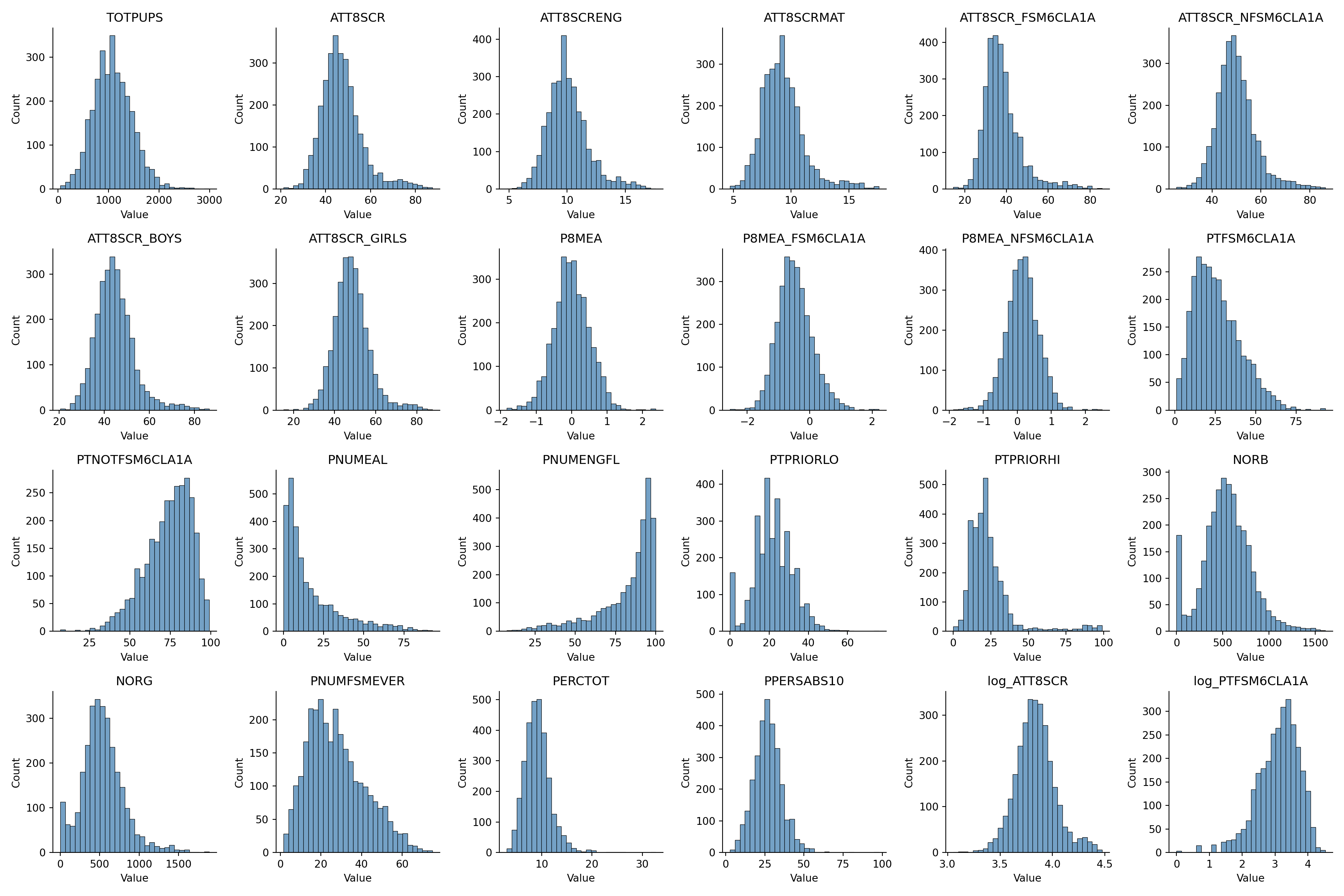
for i, var in enumerate(variables):
sns.histplot(data=numeric_long[numeric_long['variable'] == var], x='value', bins=30, color='steelblue', ax=axes[i])
axes[i].set_title(var)
axes[i].set_xlabel("Value")
axes[i].set_ylabel("Count")
# Hide unused subplots
for j in range(i + 1, len(axes)):
fig.delaxes(axes[j])
plt.tight_layout()
plt.suptitle("Histograms of Numerical Variables", y=1.02)
sns.despine()
plt.show()
```
```{python}
#| message: false
#| warning: false
import pandas as pd
import seaborn as sns
import matplotlib.pyplot as plt
import numpy as np
# Log-transform relevant variables
england_filtered_clean['log_ATT8SCR'] = np.log(england_filtered_clean['ATT8SCR'])
england_filtered_clean['log_PTFSM6CLA1A'] = np.log(england_filtered_clean['PTFSM6CLA1A'])
england_filtered_clean['log_PNUMEAL'] = np.log(england_filtered_clean['PNUMEAL'])
england_filtered_clean['log_PERCTOT'] = np.log(england_filtered_clean['PERCTOT'])
# Prepare long format data
long_df = pd.melt(
england_filtered_clean,
id_vars=['log_ATT8SCR'],
value_vars=['log_PTFSM6CLA1A', 'log_PNUMEAL', 'log_PERCTOT', 'PTPRIORLO'],
var_name='predictor',
value_name='x_value'
)
# Custom axis labels
axis_labels = {
'log_PTFSM6CLA1A': 'log(PTFSM6CLA1A)',
'log_PNUMEAL': 'log(PNUMEAL)',
'log_PERCTOT': 'log(PERCTOT)',
'PTPRIORLO': 'PTPRIORLO'
}
# Set up the figure manually
predictors = long_df['predictor'].unique()
cols = 2
rows = (len(predictors) + cols - 1) // cols
fig, axes = plt.subplots(rows, cols, figsize=(12, 4 * rows))
axes = axes.flatten()
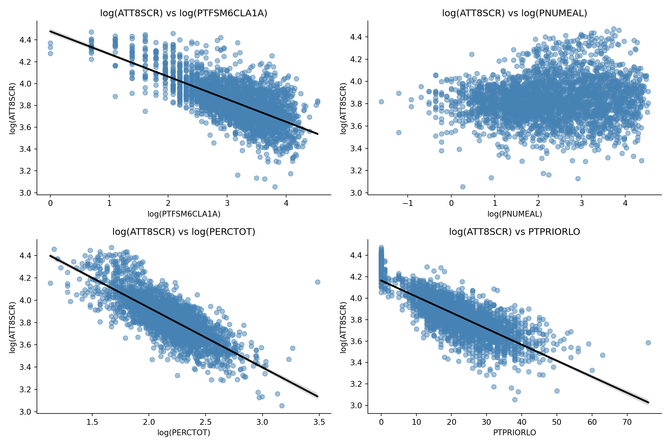
for i, predictor in enumerate(predictors):
subset = long_df[long_df['predictor'] == predictor]
sns.regplot(
data=subset,
x='x_value',
y='log_ATT8SCR',
scatter_kws={'alpha': 0.5, 'color': 'steelblue'},
line_kws={'color': 'black'},
ax=axes[i]
)
axes[i].set_title(f"log(ATT8SCR) vs {axis_labels[predictor]}")
axes[i].set_xlabel(axis_labels[predictor])
axes[i].set_ylabel("log(ATT8SCR)")
# Hide unused subplots
for j in range(i + 1, len(axes)):
fig.delaxes(axes[j])
plt.tight_layout()
plt.suptitle("Scatter Plots of log(ATT8SCR) vs Predictors", y=1.02)
sns.despine()
plt.show()
```
```{python}
#| message: false
#| warning: false
#| fig-width: 8
#| fig-height: 14
import pandas as pd
import seaborn as sns
import matplotlib.pyplot as plt
# Select categorical columns and drop unwanted ones
categorical_cols = england_filtered_clean.select_dtypes(include='object').drop(
columns=['URN', 'SCHNAME.x', 'LANAME', 'TOWN.x', 'SCHOOLTYPE.x'], errors='ignore'
)
# Determine layout
n_cols = 2
n_rows = (len(categorical_cols.columns) + n_cols - 1) // n_cols
fig, axes = plt.subplots(n_rows, n_cols, figsize=(12, 4 * n_rows))
axes = axes.flatten()
# Generate bar plots
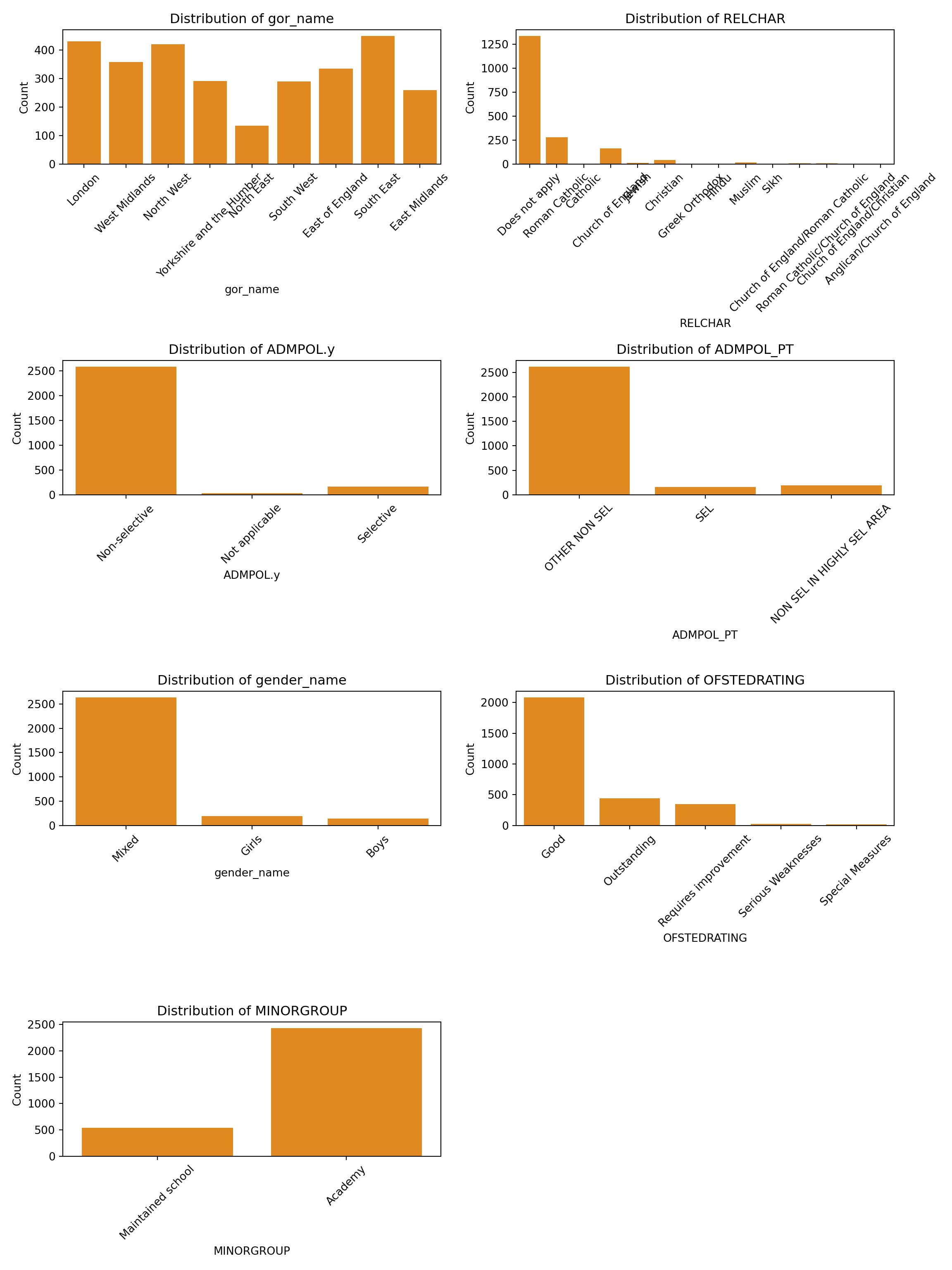
for i, colname in enumerate(categorical_cols.columns):
sns.countplot(data=categorical_cols, x=colname, ax=axes[i], color='darkorange')
axes[i].set_title(f"Distribution of {colname}")
axes[i].set_xlabel(colname)
axes[i].set_ylabel("Count")
axes[i].tick_params(axis='x', rotation=45)
# Hide unused subplots
for j in range(i + 1, len(axes)):
fig.delaxes(axes[j])
plt.tight_layout()
plt.show()
```
#### {width="41" height="30"}
```{r}
#| message: false
#| warning: false
library(tidyverse)
# Select only numeric columns
numeric_cols <- england_filtered_clean %>%
select(where(is.numeric)) %>%
select(-easting, -northing, -LEA)
# Convert to long format for faceting
numeric_long <- numeric_cols %>%
pivot_longer(cols = everything(), names_to = "variable", values_to = "value")
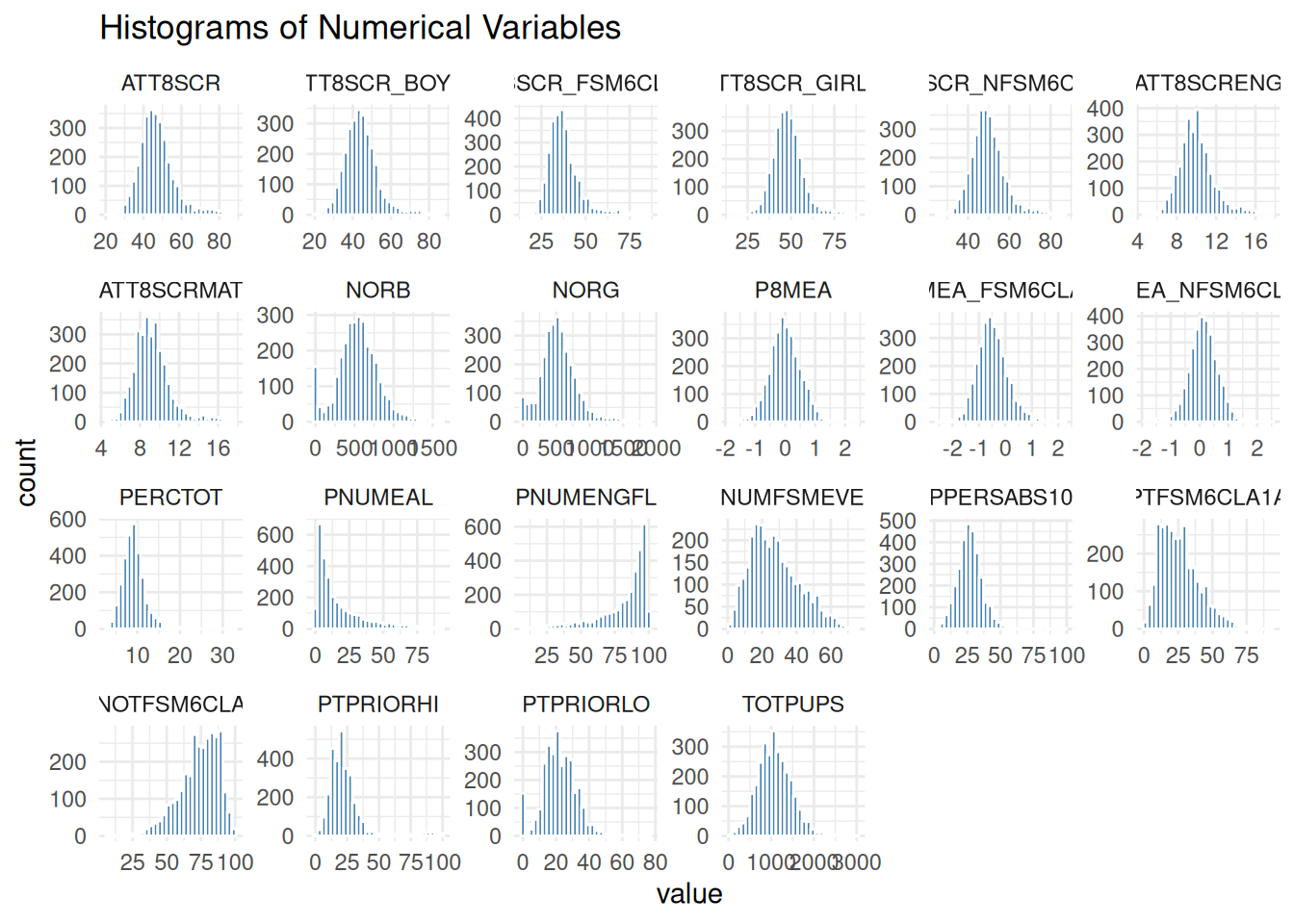
# Plot faceted histograms
ggplot(numeric_long, aes(x = value)) +
geom_histogram(bins = 30, fill = "steelblue", color = "white") +
facet_wrap(~ variable, scales = "free", ncol = 6) +
theme_minimal() +
labs(title = "Histograms of Numerical Variables")
```
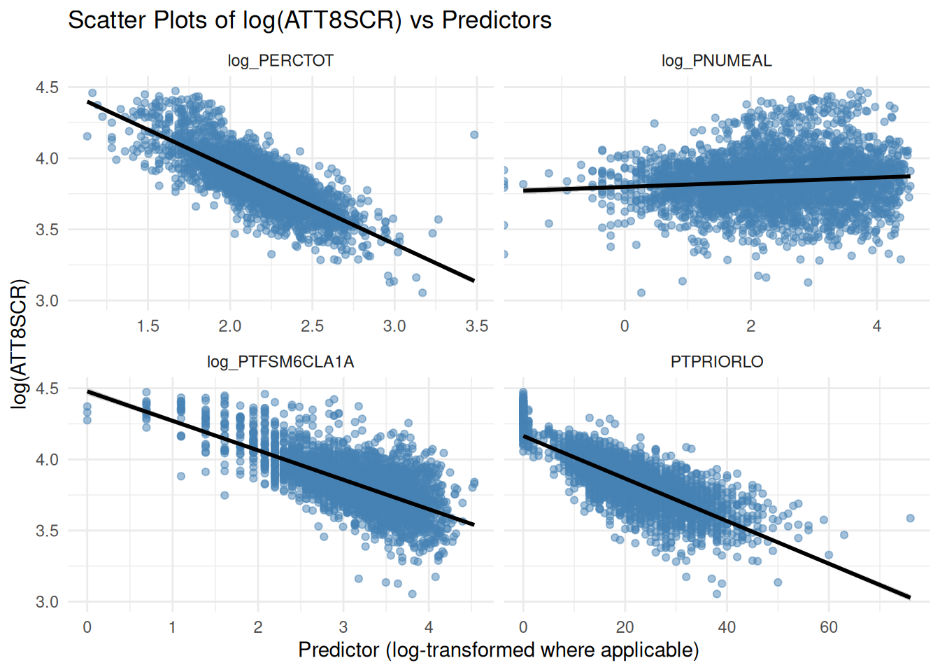
```{r}
#| message: false
#| warning: false
library(tidyverse)

# Prepare the data
scatter_data <- england_filtered_clean %>%
  select(ATT8SCR, PTFSM6CLA1A, PNUMEAL, PERCTOT, PTPRIORLO) %>%
  mutate(
    log_ATT8SCR = log(ATT8SCR),
    log_PTFSM6CLA1A = log(PTFSM6CLA1A),
    log_PNUMEAL = log(PNUMEAL),
    log_PERCTOT = log(PERCTOT)
  ) %>%
  pivot_longer(
    cols = c(log_PTFSM6CLA1A, log_PNUMEAL, log_PERCTOT, PTPRIORLO),
    names_to = "predictor",
    values_to = "x_value"
  )

# Create faceted scatter plots
ggplot(scatter_data, aes(x = x_value, y = log_ATT8SCR)) +
  geom_point(alpha = 0.5, color = "steelblue") +
  geom_smooth(method = "lm", se = TRUE, color = "black") +
  facet_wrap(~ predictor, scales = "free_x") +
  theme_minimal() +
  labs(
    title = "Scatter Plots of log(ATT8SCR) vs Predictors",
    x = "Predictor (log-transformed where applicable)",
    y = "log(ATT8SCR)"
  )
```
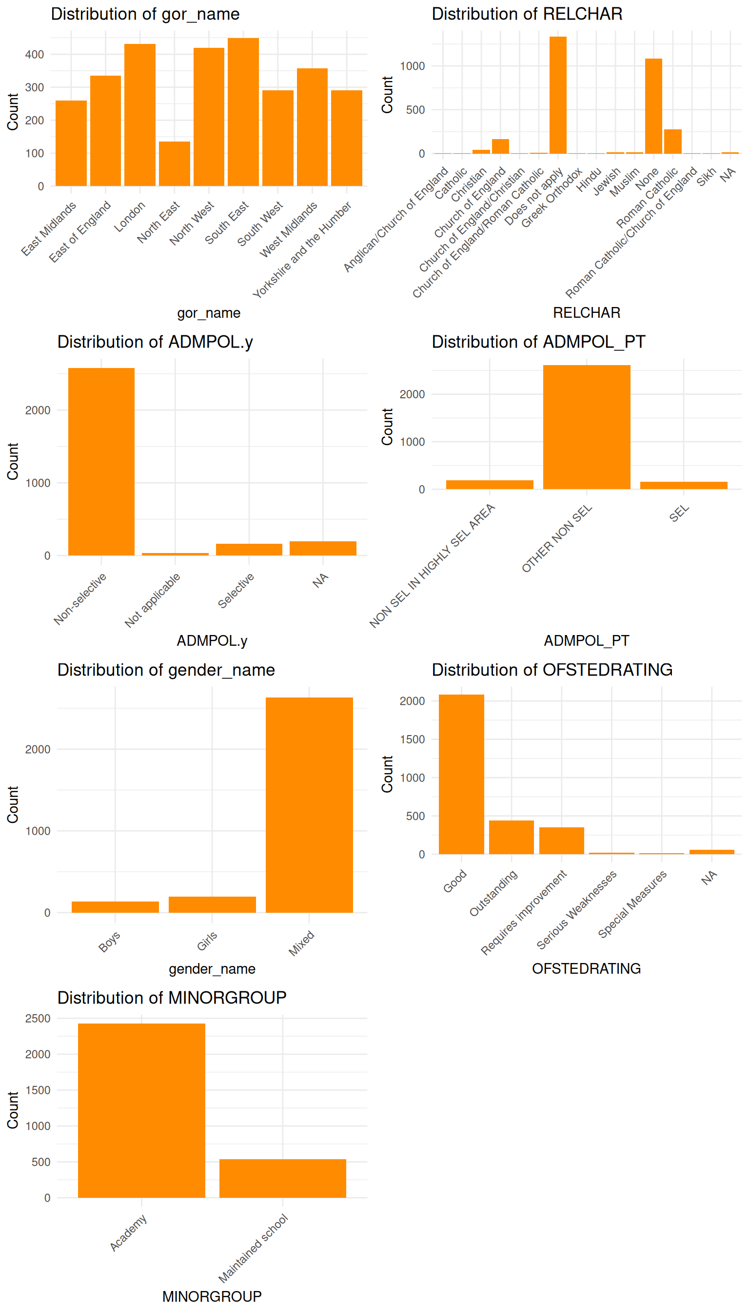
```{r}
#| message: false
#| warning: false
#| fig-width: 8
#| fig-height: 14
library(tidyverse)
library(cowplot)

# Drop unwanted columns
categorical_cols <- england_filtered_clean %>%
  select(where(is.character)) %>%
  select(-URN, -SCHNAME.x, -LANAME, -TOWN.x, -SCHOOLTYPE.x)

# Create a list to store plots (unnamed)
plot_list <- list()

# Loop through each categorical column and generate a bar plot
for (colname in names(categorical_cols)) {
  p <- ggplot(categorical_cols, aes_string(x = colname)) +
    geom_bar(fill = "darkorange") +
    theme_minimal() +
    labs(title = paste("Distribution of", colname), x = colname, y = "Count") +
    theme(axis.text.x = element_text(angle = 45, hjust = 1))

  plot_list <- append(plot_list, list(p))  # Append without naming
}

# Combine all plots into a single figure
combined_plot <- cowplot::plot_grid(plotlist = plot_list, ncol = 2)
print(combined_plot)
```
:::
### Changing your dummy reference category
Your dummy variable reference category is the category within the variable that all other categories will be compared against in your model.
While the reference category has no effect on the model itself, it does make a difference for how you interpret your model.
For example, if you are using Regions in England as a dummy, setting your reference region as London will mean all other regions are compared to it and they might naturally be lower or higher.
A good strategy is to select the most or least numerous or important category in your variable, rather than something in the middle. Of course, you may not know which is most important until you run your model, so you may need to go back and reset the reference variable and run the model again.
Here is some code in R and Python to help you carry out the setting of the reference level (Yes, it's more straightforward in R!)
::: multicode
#### {width="30"}
```{python}
#| eval: false
#| include: true
import pandas as pd
from pandas.api.types import CategoricalDtype

# Ensure it's a copy to avoid SettingWithCopyWarning
england_filtered_clean = england_filtered_clean.copy()

# Set reference level for gor_name
gor_dtype = CategoricalDtype(
    categories=["South East"] + sorted(set(england_filtered_clean["gor_name"]) - {"South East"}),
    ordered=True
)
england_filtered_clean["gor_name"] = england_filtered_clean["gor_name"].astype(gor_dtype)

# Set reference level for ofsted_rating_name
ofsted_dtype = CategoricalDtype(
    categories=["Good"] + sorted(set(england_filtered_clean["OFSTEDRATING"].dropna()) - {"Good"}),
    ordered=True
)
england_filtered_clean["ofsted_rating_name"] = england_filtered_clean["OFSTEDRATING"].astype(ofsted_dtype)

# Set reference level for ADMPOL_PT
admpol_dtype = CategoricalDtype(
    categories=["OTHER NON SEL"] + sorted(set(england_filtered_clean["ADMPOL_PT"]) - {"OTHER NON SEL"}),
    ordered=True
)
england_filtered_clean["ADMPOL_PT"] = england_filtered_clean["ADMPOL_PT"].astype(admpol_dtype)
```
#### {width="41" height="30"}
```{r}
#| message: false
#| warning: false
## In R, you can change the reference category using the relevel() function

england_filtered_clean$gor_name <- relevel(factor(england_filtered_clean$gor_name), ref = "South East")
england_filtered_clean$ofsted_rating_name <- relevel(factor(england_filtered_clean$OFSTEDRATING), ref = "Good")
england_filtered_clean$ADMPOL_PT <- relevel(factor(england_filtered_clean$ADMPOL_PT), ref = "OTHER NON SEL")
```
:::
### Reclassifying a variable into fewer categories
As mentioned in the lecture, it can sometimes be useful to reclassify a variable into fewer categories to see if a signal appears.
Let's have a look at the religious character of a school variable and test it out as dummy in a basic model:
:::{callout.note}
Note the Python code is far more complicated than the R code, but should prodice similar outputs
:::
::: multicode
#### {width="30"}
```{python}
#| message: false
#| warning: false
import numpy as np
import pandas as pd
import statsmodels.api as sm

# Drop rows with missing values in relevant columns
model_df = england_filtered_clean[['ATT8SCR', 'PTFSM6CLA1A', 'RELCHAR']].dropna().copy()

# Log-transform numeric variables
model_df['log_ATT8SCR'] = np.log(model_df['ATT8SCR'].astype(float))
model_df['log_PTFSM6CLA1A'] = np.log(model_df['PTFSM6CLA1A'].astype(float))

# Ensure RELCHAR is treated as categorical
model_df['RELCHAR'] = model_df['RELCHAR'].astype('category')

# Create design matrix with dummy variables for RELCHAR
X = pd.get_dummies(model_df[['log_PTFSM6CLA1A', 'RELCHAR']], drop_first=True)

# Add constant
X = sm.add_constant(X)

# Response variable
y = model_df['log_ATT8SCR']

# Ensure all columns are float64 to avoid dtype issues
X = X.astype('float64')
y = y.astype('float64')

# Fit linear model using Pandas DataFrame directly
model = sm.OLS(y, X).fit()

# Display summary with proper variable names
print(model.summary())
```
#### {width="41" height="30"}
```{r}
#| message: false
#| warning: false
# Fit linear model and get predicted values
england_model2 <- lm(log(ATT8SCR) ~ log(PTFSM6CLA1A) + RELCHAR, data = england_filtered_clean)
summary(england_model2)
```
:::
You will notice that the religious character variables nearly all insignificant. As such, lets try collapsing into three groups - "None", "Christian" and "Non-Christian"
::: multicode
#### {width="30"}
```{python}
#| message: false
#| warning: false
# Define mapping function
def classify_relchar(value):
    if pd.isna(value):
        return "None"
    elif value in ["Does not apply", "None"]:
        return "None"
    elif value in [
        "Roman Catholic", "Greek Orthodox", "Church of England", "Catholic", "Christian",
        "Church of England/Roman Catholic", "Roman Catholic/Church of England",
        "Church of England/Christian", "Anglican/Church of England"
    ]:
        return "Christian"
    else:
        return "Non-Christian"

# Apply classification
england_filtered_clean['RELCHAR_Grp'] = england_filtered_clean['RELCHAR'].apply(classify_relchar)
```
#### {width="41" height="30"}
```{r}
#| message: false
#| warning: false
england_filtered_clean <- england_filtered_clean %>%
  mutate(RELCHAR_Grp = case_when(
    RELCHAR %in% c("Does not apply", "None") ~ "None",
    RELCHAR %in% c(
      "Roman Catholic", "Greek Orthodox", "Church of England", "Catholic", "Christian",
      "Church of England/Roman Catholic", "Roman Catholic/Church of England",
      "Church of England/Christian", "Anglican/Church of England"
    ) ~ "Christian",
    TRUE ~ "Non-Christian"
  ))
```
:::
Now re-run your model
::: multicode
#### {width="30"}
```{python}
#| message: false
#| warning: false
import numpy as np
import pandas as pd
import statsmodels.api as sm

# Convert RELCHAR_Grp to a categorical variable with "None" as the reference level
england_filtered_clean['RELCHAR_Grp'] = pd.Categorical(
    england_filtered_clean['RELCHAR_Grp'],
    categories=["None", "Christian", "Non-Christian"],
    ordered=False
)

# Drop rows with missing values in relevant columns
model_df = england_filtered_clean[['ATT8SCR', 'PTFSM6CLA1A', 'RELCHAR_Grp']].dropna().copy()

# Log-transform numeric variables
model_df['log_ATT8SCR'] = np.log(model_df['ATT8SCR'].astype(float))
model_df['log_PTFSM6CLA1A'] = np.log(model_df['PTFSM6CLA1A'].astype(float))

# Ensure RELCHAR is treated as categorical
model_df['RELCHAR_Grp'] = model_df['RELCHAR_Grp'].astype('category')

# Create design matrix with dummy variables for RELCHAR
X = pd.get_dummies(model_df[['log_PTFSM6CLA1A', 'RELCHAR_Grp']], drop_first=True)

# Add constant
X = sm.add_constant(X)

# Response variable
y = model_df['log_ATT8SCR']

# Ensure all columns are float64 to avoid dtype issues
X = X.astype('float64')
y = y.astype('float64')

# Fit linear model using Pandas DataFrame directly
model = sm.OLS(y, X).fit()

# Display summary with proper variable names
print(model.summary())
```
#### {width="41" height="30"}
```{r}
#| message: false
#| warning: false
# Fit linear model and get predicted values
# Ensure RELCHAR_Grp is a factor with "None" as the reference level
england_filtered_clean <- england_filtered_clean %>%
  mutate(RELCHAR_Grp = factor(RELCHAR_Grp, levels = c("None", "Christian", "Non-Christian")))

england_model2 <- lm(log(ATT8SCR) ~ log(PTFSM6CLA1A) + RELCHAR_Grp, data = england_filtered_clean)
summary(england_model2)
```
:::
Has this made a difference? What's happened to the significance of the religious character variable?
:::{.callout-tip}
You can use this method to reclassify any different variable.
Think about how you might reclassify a continuous variable. You might think about converting something like 'total number of pupils on roll' into 'small', 'medium' and 'large' schools, for example, based on certain thresholds. How might you choose these thresholds? If you are struggling to think of how you might code this kind of reclassification up, this is exactly where AI can be very helpful in assisting you - although while it might be good at the code to do it, I can guarantee it will likely be pretty bad at deciding on useful breaks in your data, so this is where you might need to intervene.
:::
## Task 3 - Building your optimum multiple regression model
### Recipe Steps
- Using the steps you learned last week and the information from this week's lecture, I would like you to find the best possible ***7-dependent variable model*** for your chosen attainment variable (without interaction terms). These can be continuous or categorical variables or any combination of them. Remember:
- Use exploratory analysis to check the distributions of your variables using histograms, box plots etc. or binary scatter plots with your dependent variable, ***before*** putting them into your model (you've already done some of this, but you may need to do some more)
- you might run into issues with logging some variables that have real 0s in them - this might cause your model to break. You might need to filter these variables out of your dataset before running your model. Some of the code above will help with this - if you get stuck, ask a friendly AI for help
- with your dummy variables, you might want to experiment with changing your reference category
- you might also want to reclassify a variable if you suspect it is important, but that in its present form is coming out as insignificant
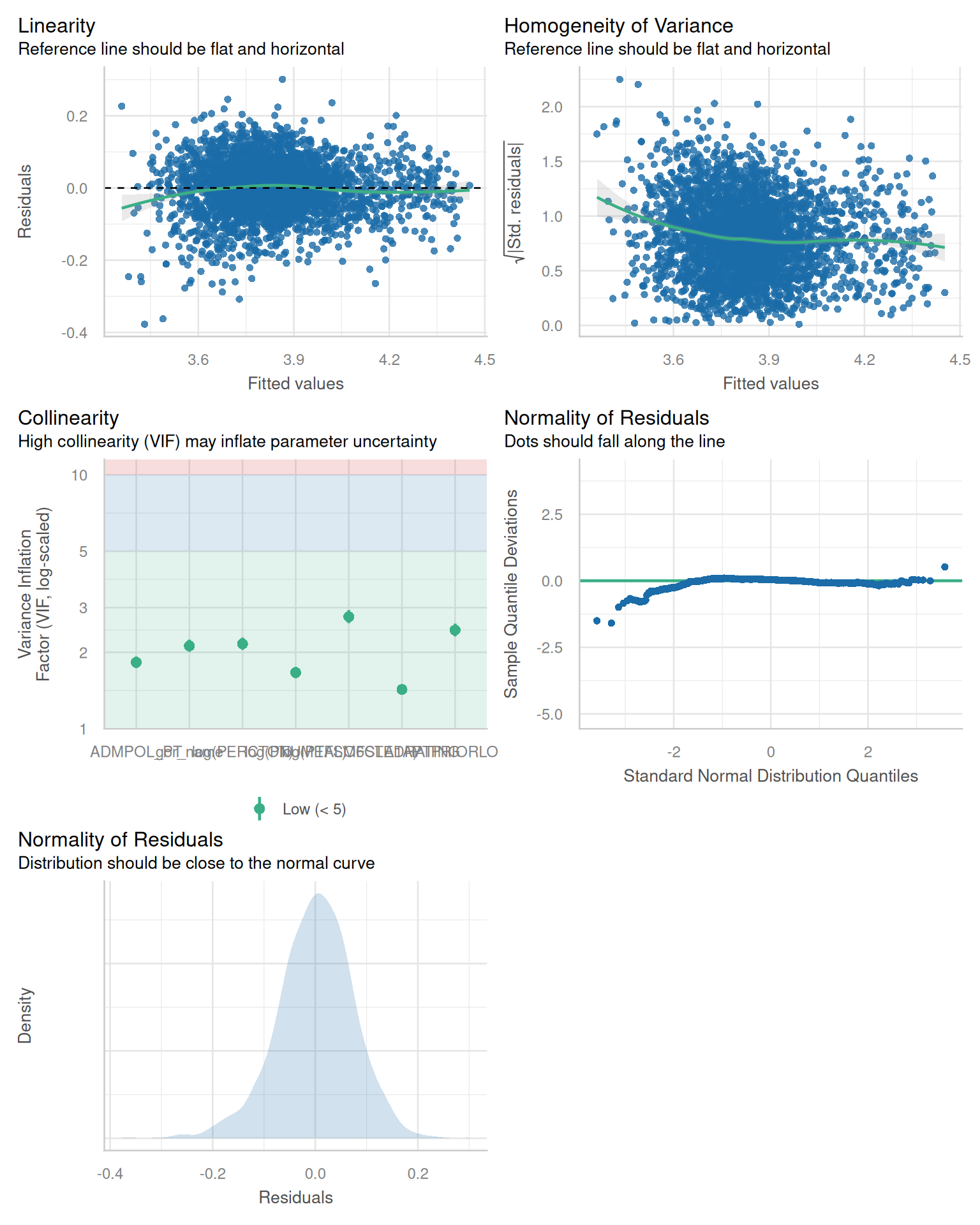
- check you regression assumptions - linearity, homoscedasticity, normality of residuals, multicollinearity, independence of residuals - does your model pass?
- which are the most important variables in your model in terms of t-values?
- You should try and build your model step by step, a variable at a time. Each time you run the model, check what is happening to the coefficients
- What do you notice about confounding or mediation as you go?
- Do any of your variables become insignificant? For example, what happens to religious character groups in the presence of regions, for example? If a variable becomes insignificant, you might we wise to drop it from the analysis (but maybe not until the end in case another variable makes it significant again)
#### ON YOUR MARKS, GET SET - GO!!!
When you think you have your best model, move on to Task 4 below
::: multicode
#### {width="30"}
```{python}
#| message: false
#| warning: false
import numpy as np
import statsmodels.formula.api as smf

# Filter rows where all log-transformed variables are > 0
england_filtered_clean = england_filtered_clean[
    (england_filtered_clean['PTFSM6CLA1A'] > 0) &
    (england_filtered_clean['PERCTOT'] > 0) &
    (england_filtered_clean['PNUMEAL'] > 0)
].copy()

# Create log-transformed columns
england_filtered_clean['log_ATT8SCR'] = np.log(england_filtered_clean['ATT8SCR'])
england_filtered_clean['log_PTFSM6CLA1A'] = np.log(england_filtered_clean['PTFSM6CLA1A'])
england_filtered_clean['log_PERCTOT'] = np.log(england_filtered_clean['PERCTOT'])
england_filtered_clean['log_PNUMEAL'] = np.log(england_filtered_clean['PNUMEAL'])

# Fit the model
model = smf.ols(
    formula='log_ATT8SCR ~ log_PTFSM6CLA1A + log_PERCTOT + log_PNUMEAL + OFSTEDRATING + gor_name + PTPRIORLO + ADMPOL_PT',
    data=england_filtered_clean
).fit()

print(model.summary())
```
#### {width="41" height="30"}
```{r}
#| message: false
#| warning: false
library(performance)
library(jtools)

england_filtered_clean <- england_filtered_clean %>%
  filter(PTFSM6CLA1A > 0, PERCTOT > 0, PNUMEAL > 0)

england_model3 <- lm(log(ATT8SCR) ~ log(PTFSM6CLA1A) + log(PERCTOT) + RELCHAR_Grp, data = england_filtered_clean)
summary(england_model3)
england_model4 <- lm(log(ATT8SCR) ~ log(PTFSM6CLA1A) + log(PERCTOT) + gor_name, data = england_filtered_clean, na.action = na.exclude)
summary(england_model4)
england_model5 <- lm(log(ATT8SCR) ~ log(PTFSM6CLA1A) + log(PERCTOT) + log(PNUMEAL) + gor_name, data = england_filtered_clean, na.action = na.exclude)
summary(england_model5)
england_model6 <- lm(log(ATT8SCR) ~ log(PTFSM6CLA1A) + log(PERCTOT) + log(PNUMEAL) + OFSTEDRATING + gor_name, data = england_filtered_clean, na.action = na.exclude)
summary(england_model6)
england_model7 <- lm(log(ATT8SCR) ~ log(PTFSM6CLA1A) + log(PERCTOT) + log(PNUMEAL) + OFSTEDRATING + gor_name + PTPRIORLO + ADMPOL_PT, data = england_filtered_clean, na.action = na.exclude)
summary(england_model7)
#Get fitted values with NA for excluded rows
fitted_vals <- fitted(england_model7)

# Add fitted values to the dataframe
england_filtered_clean$fitted7 <- fitted_vals
```
:::
## Task 4 - Evaluation
- When you have your 'best' model, how do you interpret the coefficients?
- Which variable(s) has(have) the most explanatory power (check t-values for this)?
- How do you interpret the combined explanatory power of variables in your model?
- What kind of confounding do you observe as you add more variables (if any)?
- Do you have any issues of multicollinearity or residual independence? Does your model pass the standard tests?
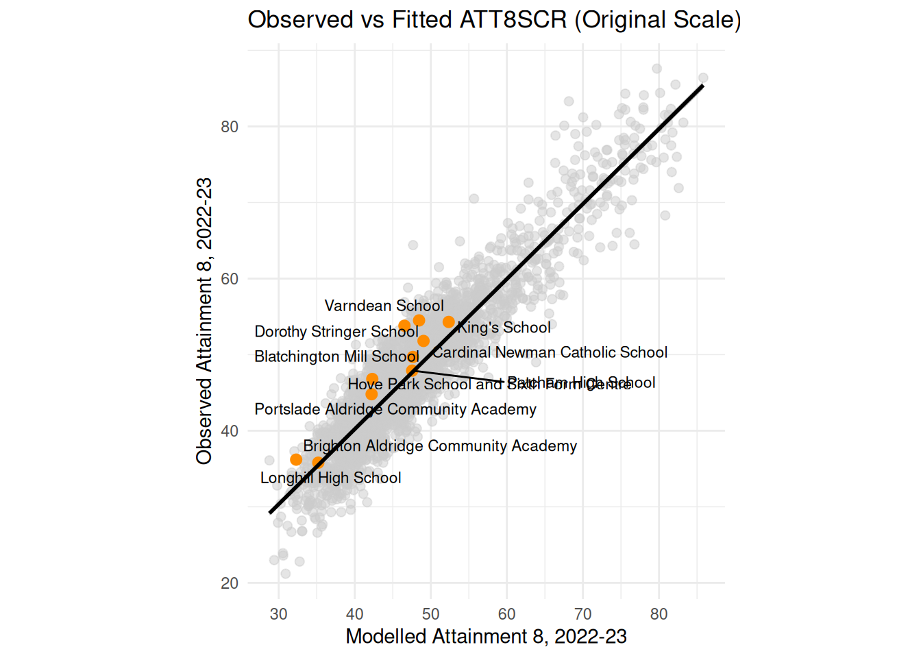
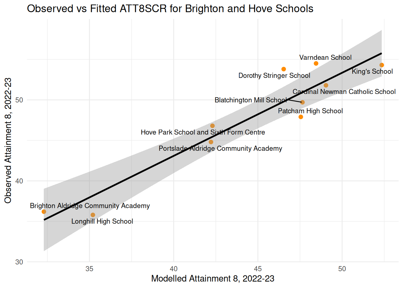
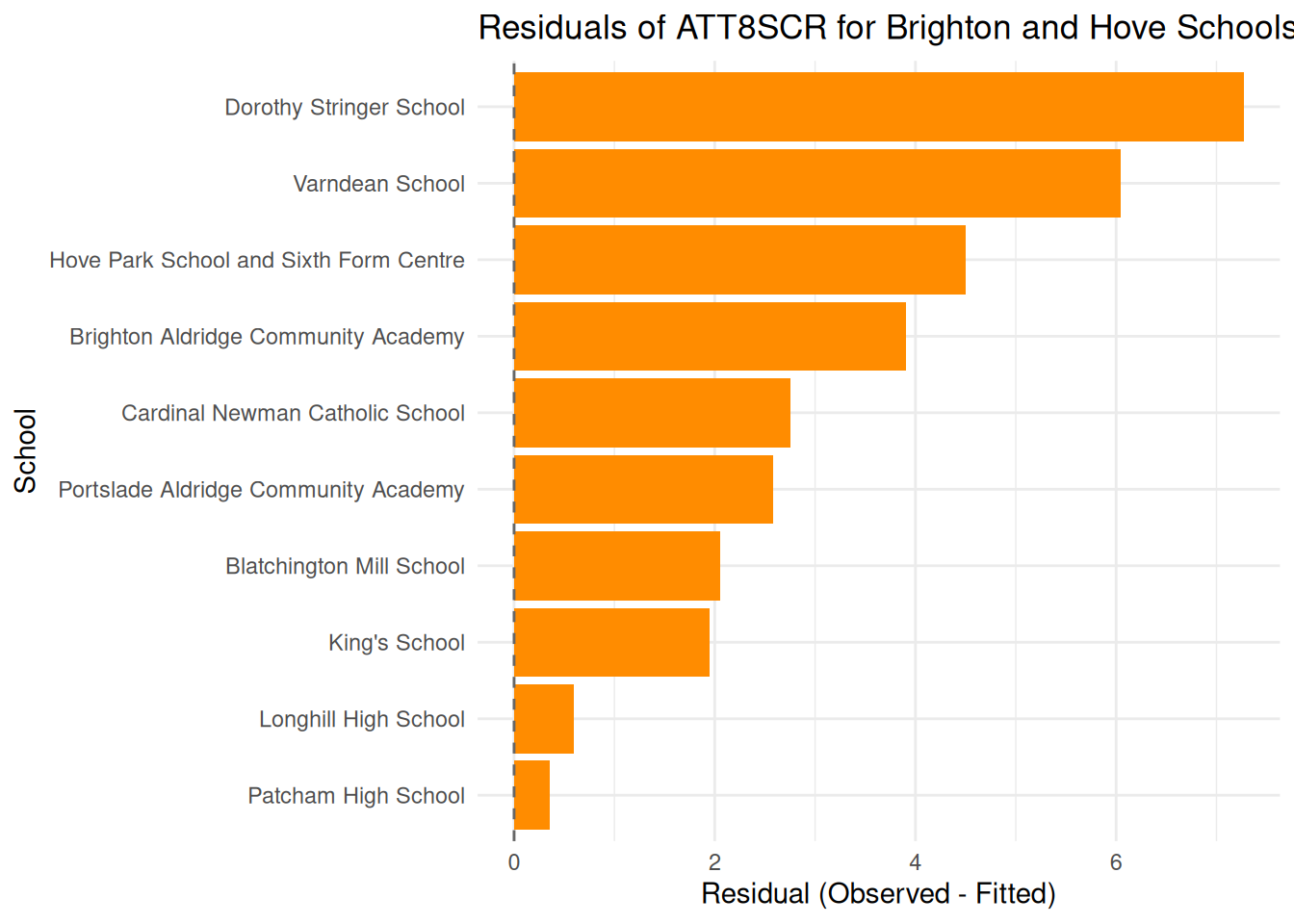
- You should also plot your model estimates (fitted values) against your original $Y$ variable as I have done below (possibly overlay your local authorities from last week as well) and map your residuals too.
Here's my best model in R compared with some of the others I built as I went along:
```{r}
names(coef(england_model3))
coef_names <- c(
  "Constant" = "(Intercept)",
  #"Religious Christian" = "RELCHAR_GrpChristian",
  #"Religious not-Christian","RELCHAR_GrpNon-Christian",
  "% Disadvantaged end KS4 (log)" = "log(PTFSM6CLA1A)",
  "% overall absence (log)" = "log(PERCTOT)",
  "% English Not First Language (log)" = "log(PNUMEAL)",
  "Ofsted: Outstanding" = "OFSTEDRATINGOutstanding",
  "Ofsted: Requires Improvement" = "OFSTEDRATINGRequires improvement",
  "Ofsted: Serious Weaknesses" = "OFSTEDRATINGSerious Weaknesses",
  "Ofsted: Special Measures" = "OFSTEDRATINGSpecial Measures",
  "Region: East Midlands" = "gor_nameEast Midlands",
  "Region: East of England" = "gor_nameEast of England",
  "Region: London" = "gor_nameLondon",
  "Region: North East" = "gor_nameNorth East",
  "Region: North West" = "gor_nameNorth West",
  "Region: South West" = "gor_nameSouth West",
  "Region: West Midlands" = "gor_nameWest Midlands",
  "Region: Yorkshire and the Humber" = "gor_nameYorkshire and the Humber",
  "% Low Prior Attainment" = "PTPRIORLO",
  "Admissions: Non-selective in Highly Selective Area" = "ADMPOL_PTNON SEL IN HIGHLY SEL AREA",
  "Admissions: Selective" = "ADMPOL_PTSEL"
)
```
```{r}
library(jtools)

export_summs(
  england_model3, england_model4, england_model5, england_model6, england_model7,
  robust = "HC3",
  coefs = coef_names
)
```
```{r}
#| fig-width: 8
#| fig-height: 10
check_model(england_model7)
```
```{r}
#| message: false
#| warning: false
library(tidyverse)
library(ggrepel)

# Convert fitted values back to original scale
england_filtered_clean <- england_filtered_clean %>%
  mutate(
    fitted_original = exp(fitted7),
    highlight = LANAME == "Brighton and Hove",
    label = if_else(highlight, SCHNAME.x, NA_character_)
  )

# Scatter plot with layered points and full-model fit line
ggplot(england_filtered_clean, aes(x = fitted_original, y = ATT8SCR)) +
  # All schools in grey
  geom_point(color = "grey80", alpha = 0.5, size = 2) +

  # Brighton and Hove schools in orange
  geom_point(data = filter(england_filtered_clean, highlight),
             aes(x = fitted_original, y = ATT8SCR),
             color = "darkorange", size = 2.5) +

  # Labels for Brighton and Hove schools
  geom_text_repel(data = filter(england_filtered_clean, highlight),
                  aes(label = label),
                  size = 3, max.overlaps = 20) +

  # Line of best fit for all schools
  geom_smooth(method = "lm", se = TRUE, color = "black") +

# Mirror x and y axes
  coord_equal() +


  theme_minimal() +
  labs(
    title = "Observed vs Fitted ATT8SCR (Original Scale)",
    x = "Modelled Attainment 8, 2022-23",
    y = "Observed Attainment 8, 2022-23"
  )
```
```{r}
#| message: false
#| warning: false
# Filter for Brighton and Hove only
brighton_data <- england_filtered_clean %>%
  filter(LANAME == "Brighton and Hove")

# Plot with regression line
ggplot(brighton_data, aes(x = fitted_original, y = ATT8SCR)) +
  geom_point(color = "darkorange", size = 2) +
  geom_smooth(method = "lm", se = TRUE, color = "black") +
  geom_text_repel(aes(label = SCHNAME.x), max.overlaps = 20, size = 3) +
  theme_minimal() +
  labs(
    title = "Observed vs Fitted ATT8SCR for Brighton and Hove Schools",
    x = "Modelled Attainment 8, 2022-23",
    y = "Observed Attainment 8, 2022-23"
  )
```
```{r}
#| message: false
#| warning: false
library(tidyverse)

# Calculate residuals and filter for Brighton and Hove
brighton_residuals <- england_filtered_clean %>%
  filter(LANAME == "Brighton and Hove") %>%
  mutate(
    fitted_original = exp(fitted7),
    residual = ATT8SCR - fitted_original,
    abs_residual = abs(residual)
  )

# Create a bar plot centered on zero
ggplot(brighton_residuals, aes(x = reorder(SCHNAME.x, residual), y = residual)) +
  geom_col(fill = "darkorange") +
  geom_hline(yintercept = 0, linetype = "dashed", color = "grey40") +
  coord_flip() +
  theme_minimal() +
  labs(
    title = "Residuals of ATT8SCR for Brighton and Hove Schools",
    x = "School",
    y = "Residual (Observed - Fitted)"
  )
```
## Task 5 - Interacting Variables (Extension activity)
In the lecture, you saw how we could look at how some of the continuous variables (like disadvantage or absence) vary by categorical variable levels (like region). Or indeed, whether continuous variables might interact with each other - for example do levels of unauthorised absence and disadvantage affect each other.
As you saw in the lecture, interpreting interactions can be complex, so here I would just like you to have a brief experiment with some of the variables in your best model.
If you are struggling to understand these effects, again, an AI helper like Gemini or ChatGPT might help you understand these interactions if you feed it your model outputs.
Most of the time in most of the regression models you build, you might not need to interact variables, but it can be informative. Next week, however, we will look at other alternatives to interacting variables when we move onto linear mixed effects models. So at this point, just some experimentation is what I would like you to achieve.