Prof D’s Regression Sessions - Vol 2
Time to go even deeper!
Adam Dennett - a.dennett@ucl.ac.uk
1st August 2024
CASA0007 Quantitative Methods
This week’s Session Aims
- Build on the basics you learned last week and learn how to extend regression modelling into multiple dimensions
- Understand the main benefits, risks and steps to take when gradually building the complexity of your models
- Understand who to interpret the outputs correctly
- Gain an appreciation of how regression help explain the phenomena we are observing
- Have hands-on practice at building and interpreting your own complex models
Recap - Last Week’s Model
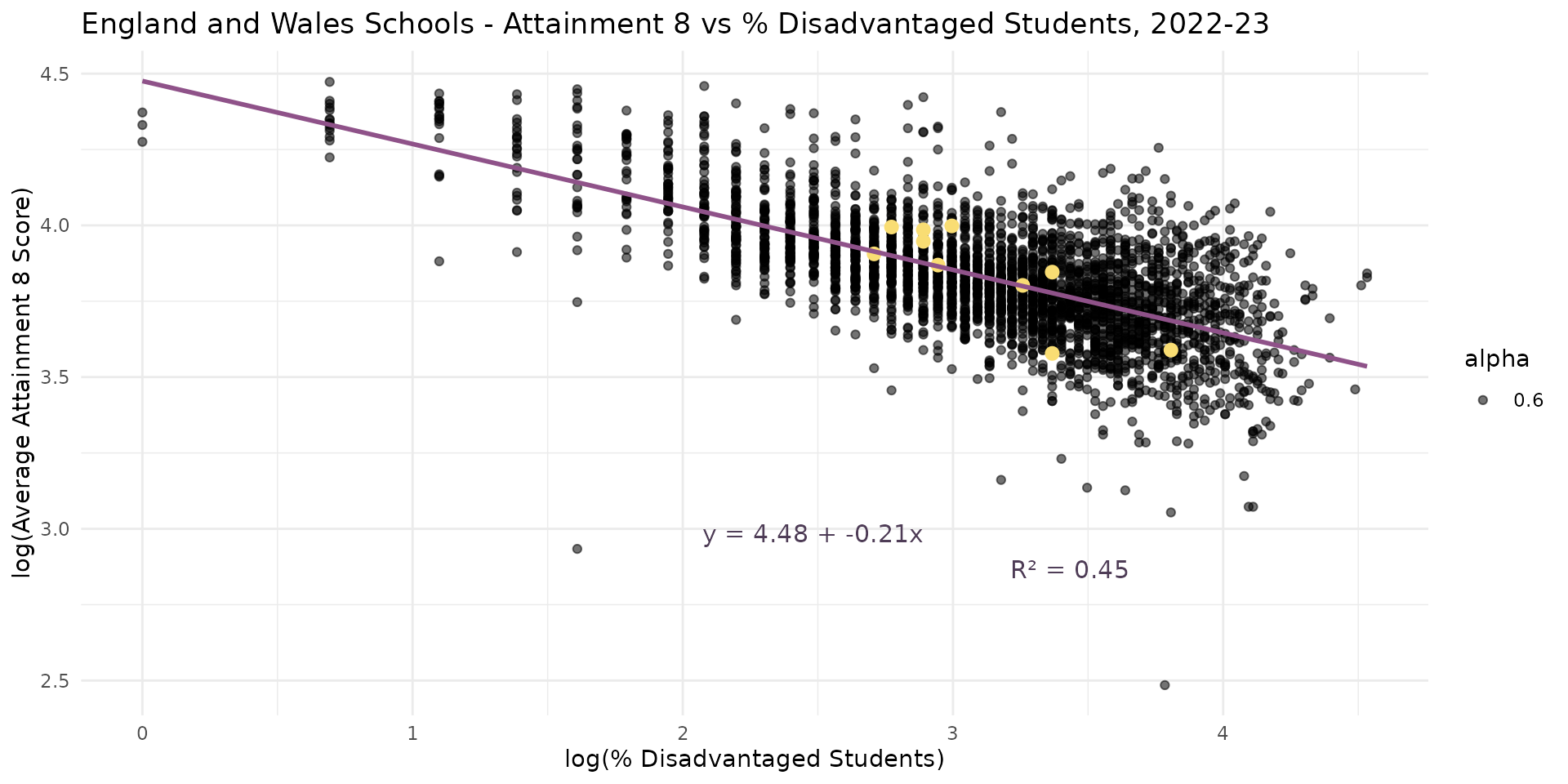
- Work of Gorard suggested link between levels of disadvantage in a school and attainment.
- Not a linear relationship but a log-log elasticity
Recap - Last Week’s Model
- School-level relationship between attainment and disadvantage unreliable at the local authority level with small changes influencing coefficients where degrees of freedom are low
An Alternative Model
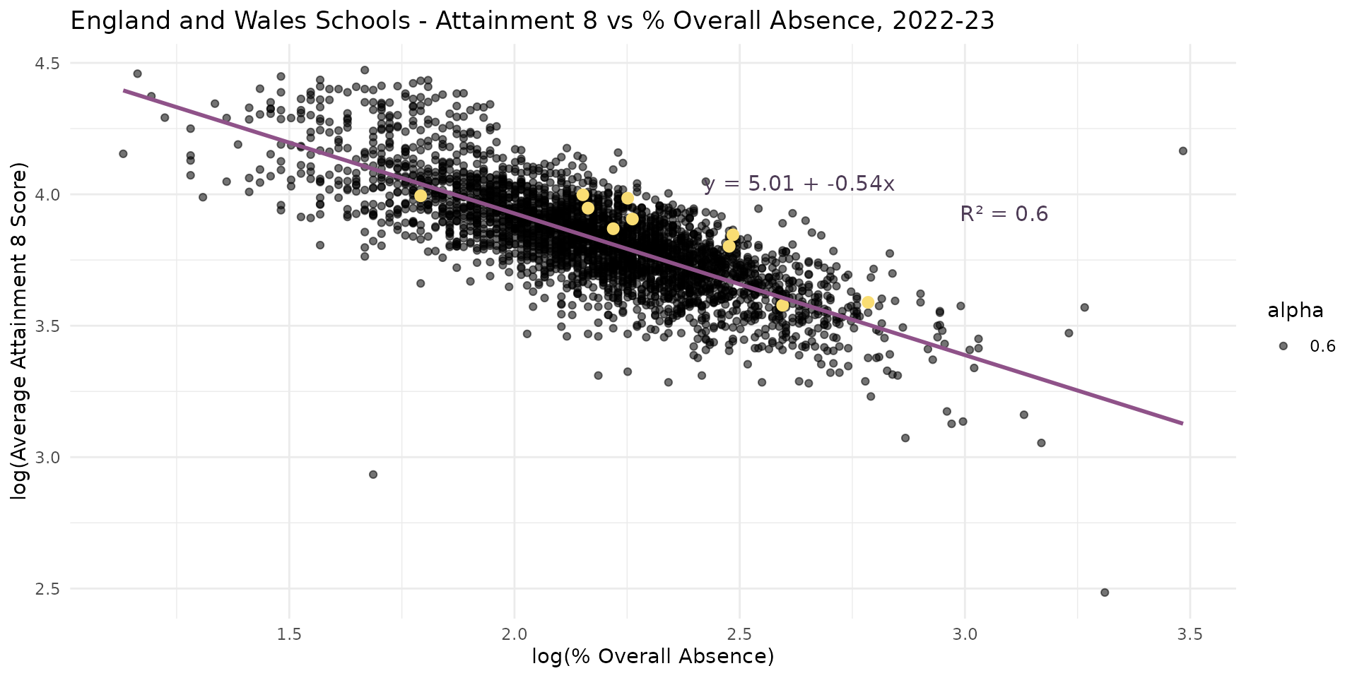
- Other research suggests overall levels of absence might be even more important
- How can we tell for sure?
An Alternative Model
Call:
lm(formula = log(ATT8SCR) ~ log(PERCTOT), data = england_filtered)

Residuals:
     Min       1Q   Median       3Q      Max
-1.16241 -0.07336  0.00471  0.07247  1.03789

Coefficients:
             Estimate Std. Error t value Pr(>|t|)
(Intercept)   5.00521    0.01712  292.40   <2e-16 ***
log(PERCTOT) -0.53898    0.00778  -69.27   <2e-16 ***
---
Signif. codes:  0 '***' 0.001 '**' 0.01 '*' 0.05 '.' 0.1 ' ' 1

Residual standard error: 0.1223 on 3231 degrees of freedom
  (15 observations deleted due to missingness)
Multiple R-squared:  0.5976,    Adjusted R-squared:  0.5975
F-statistic:  4799 on 1 and 3231 DF,  p-value: < 2.2e-16
- Overall Absence = bigger coefficient (-0.54 vs -0.21) & improves the \(R^2\) to (60% vs 45% for the % disadvantage model)
- Suggests that Overall Absence explains more variation in Attainment 8
Multiple Linear Regression
- One way to really tell which variable is more important is to put them in a model together and observe how the affect each other
- Multiple linear regression extends bivariate regression to include multiple independent variables
- As with bivariate regression, variables should be chosen based on theory and prior research rather than just throwing the variables in because you have them
- However, it’s permissible to explore relationships and experiment and iterate between data exploration and theory - both can inform each other
Multiple Linear Regression
- When we start adding more variables into the model, an alternative to the mode generic notation is to include the variables in the equation explicitly, for example:
\[\log(\text{Attainment8}) = \beta_0 + \beta_1\log(\text{PctDisadvantage}) +\\\\ \beta_2log(\text{PctPersistentAbsence}) + \epsilon\]
- There’s no real limit to the number of variables you can include in a model - however:
- Fewer is easier to interpret
- More variables will reduce your degrees of freedom
Multiple Linear Regression
Multiple Linear Regression
Call:
lm(formula = log(ATT8SCR) ~ log(PTFSM6CLA1A) + log(PERCTOT),
    data = model_data)

Residuals:
     Min       1Q   Median       3Q      Max
-1.26481 -0.06531 -0.00040  0.06352  0.77403

Coefficients:
                  Estimate Std. Error t value Pr(>|t|)
(Intercept)       5.063088   0.015126  334.72   <2e-16 ***
log(PTFSM6CLA1A) -0.111473   0.003578  -31.16   <2e-16 ***
log(PERCTOT)     -0.406199   0.008045  -50.49   <2e-16 ***
---
Signif. codes:  0 '***' 0.001 '**' 0.01 '*' 0.05 '.' 0.1 ' ' 1

Residual standard error: 0.1072 on 3230 degrees of freedom
Multiple R-squared:  0.6906,    Adjusted R-squared:  0.6904
F-statistic:  3605 on 2 and 3230 DF,  p-value: < 2.2e-16
- What is the model telling us?
Multiple Linear Regression
| 19500.8 |
19500.8 |
19525.1 |
0.69 |
0.69 |
0.11 |
0.11 |
Multiple Linear Regression
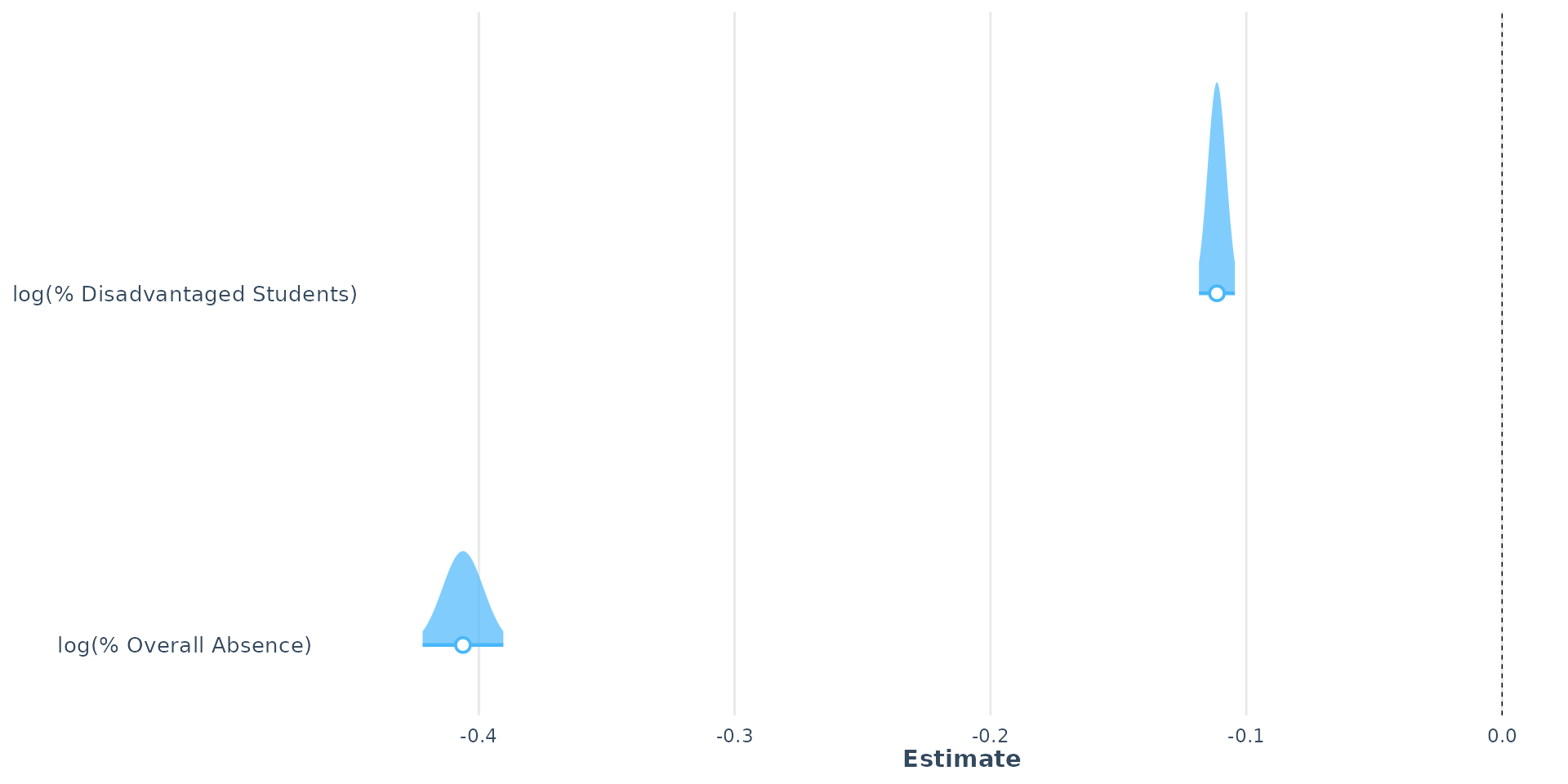
- The coefficients for both variables are statistically significant and negative, indicating that both variables contribute to explaining the variation in Attainment 8 scores
- But t-values indicate that the % Overall Absence variable (-50.49) has a stronger effect on Attainment 8 scores than the % Disadvantaged Students variable (-31.16)
- The \(R^2\) value is now 0.69, indicating that the model is potentially good and explains 69% of the variation in Attainment 8 scores. Degrees of freedom are good and the overall model is statistically significant.
- But does is satisfy the assumptions of linear regression?
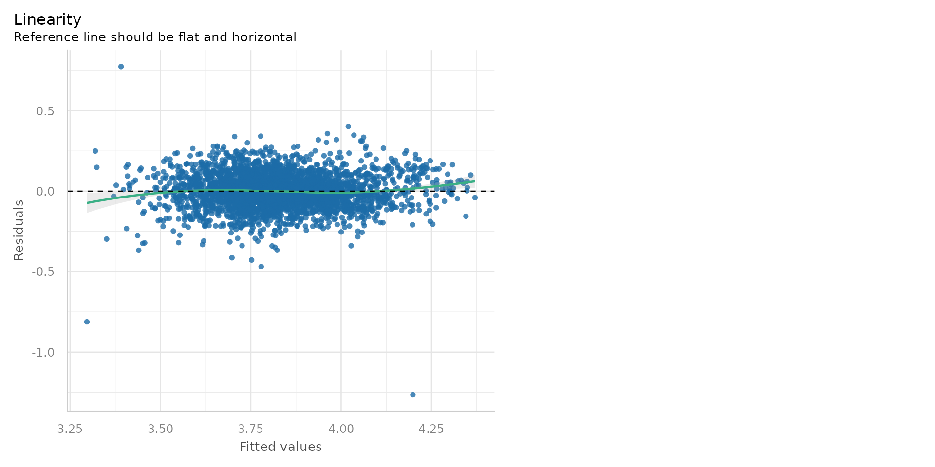
Diagnostics 1
- Pretty good - the residuals are randomly scattered around zero, suggesting a linear relationship
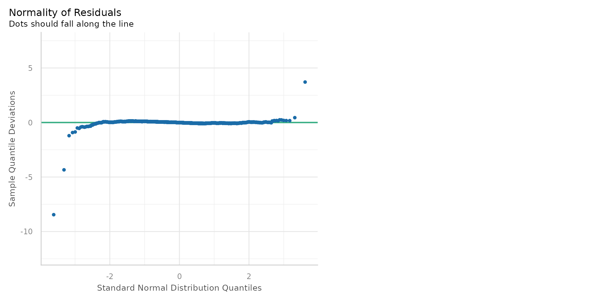
Diagnostics 2
- The residuals are normally distributed - the Q-Q plot shows most points on the line
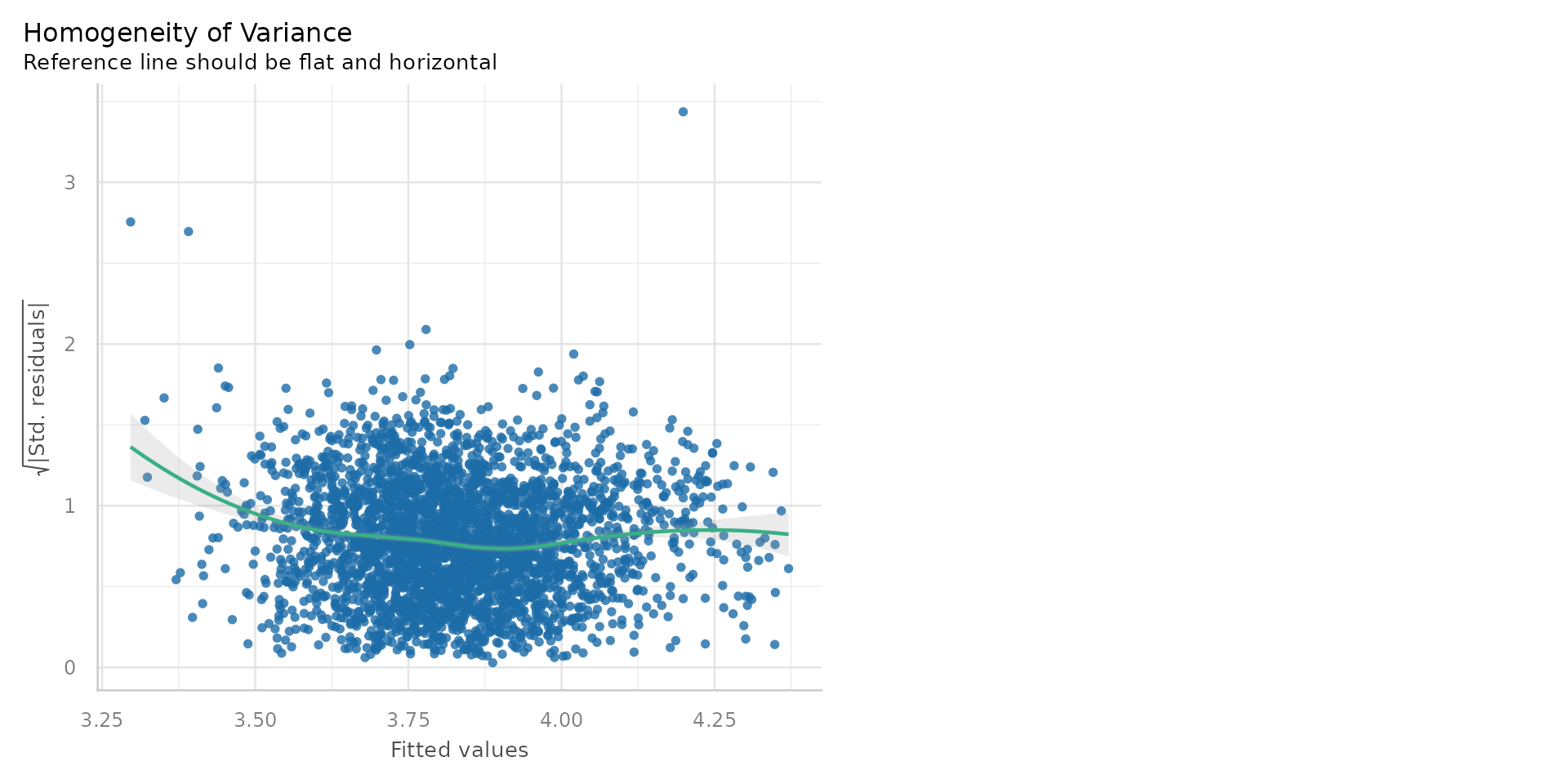
Diagnostics 3
- The residuals are randomly scattered around zero, suggesting constant variance.
Linear Regression - Diagnostics
- Linearity: 😎
- Homoscedasticity: 😎
- Normality of residuals: 😎
- No multicollinearity: 😕
- Independence of residuals: 😕
Multicollinearity
- Multicollinearity occurs when two or more independent variables in a regression model are highly correlated with each other
- This can lead to unreliable estimates of the coefficients, inflated standard errors, and difficulty in interpreting the results
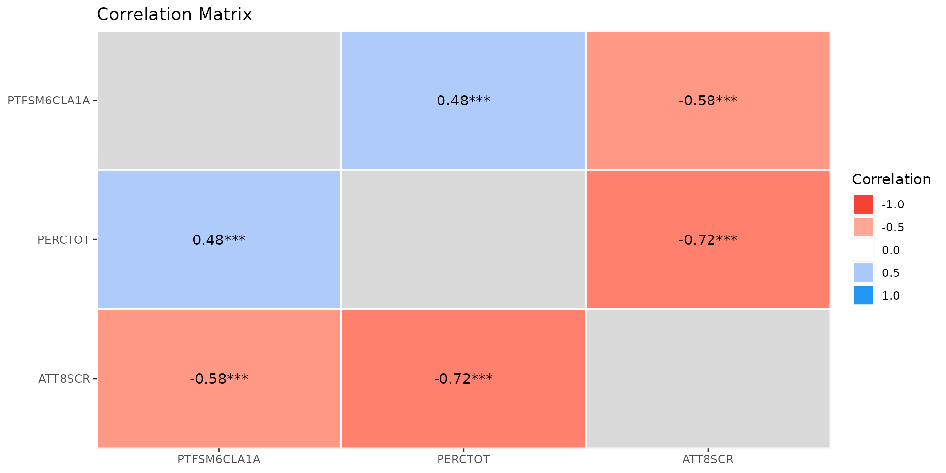
Multicollinearity
- A quick and easy way to check for the correlation between your independent variables is generate a standard correlation matrix/plot
- Difficult to say what is too much correlation - but over 0.7 is often considered problematic
- However, pairwise correlations might miss n-way correlations
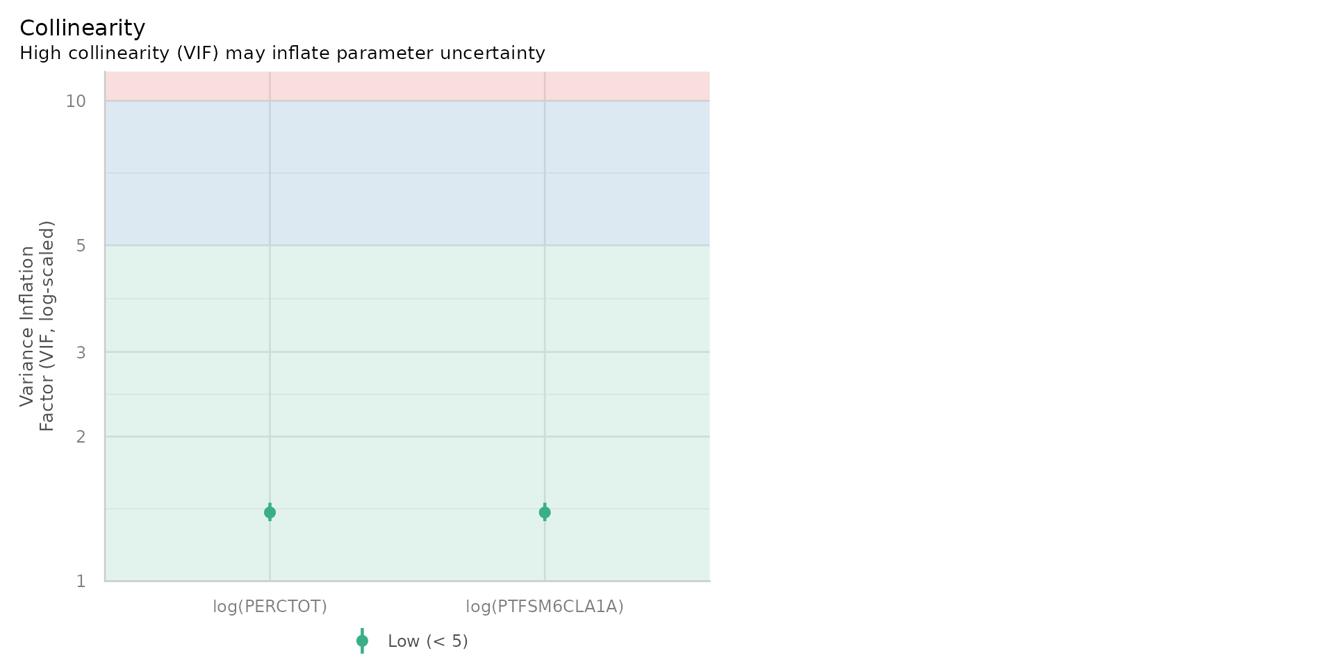
Variance Inflaction Factor - VIF
- A more useful diagnostic tool is the Variance Inflation Factor (VIF), which measures how much the variance of a regression coefficient is increased due to multicollinearity
- A VIF value of 1 indicates no correlation, while a VIF value above 5 or 10 suggests high multicollinearity
Variance Inflaction Factor - VIF
Why does it even matter if the variance is inflated?
- Variance = Uncertainty in our model
- If 2 or more variables are highly correlated and both appear to affect the dependent variable, it can be difficult to determine which variable is actually having the effect
- The model makes an arbitrary split
- Small changes in the data could make the split go either way - e.g. attribute more of the effect to % Disadvantaged Students or % Overall Absence (if VIF high) - thus inflating the uncertainty / variance
Variance Inflaction Factor - VIF
- Despite some positive correlation (0.48) between % Disadvantaged Students and % Overall Absence, the VIF is very low ~1.5
- No problems with multicollinearity
- So we have passed that test and can happily use both in the model
Linear Regression - Diagnostics
- Linearity: 😎
- Homoscedasticity: 😎
- Normality of residuals: :😎:
- No multicollinearity: 😎
- Independence of residuals: 😕
Independence of Residuals
- Residuals (errors) should not be correlated with each other
- (auto)correlation (clustering) in the errors = model missing something!
- can lead to biased estimates and incorrect conclusions
- often occurs when a temporal or spatial component to the data
- or when another important variable is missing or omitted
Spatial or Temporal (auto)Correlation
- In our case, we have a spatial component to the data - schools are located in different areas of England and Wales
- If schools in the same area have similar characteristics, it is likely that the residuals will be correlated
- The easiest way to check this is to plot the values of the residuals for the schools on a map
Residual (auto)Correlation
- Residuals show clear spatial autocorrelation
- London (and other city schools) perform much better than model predicts
Residual (auto)Correlation
- ALWAYS MAP YOUR RESIDUALS IF MODELLING SPATIAL DATA
- Correlated residuals often the sign of an omitted variable (e.g “London”)
- In the GIS Course you will learn a lot more about testing for spatial autocorrelation (using Moran’s I) and how spatial variables (lags, error terms) or geographically weighted regression can be used to deal with spatial autocorrelation
- Here we will try something much simpler - adding London (and other regions) to our model
Linear Regression - Diagnostics
- Linearity: 😎
- Homoscedasticity: 😎
- Normality of residuals: :😎:
- No multicollinearity: 😎
- Independence of residuals: 😬
Dummy Variables
- In linear regression, independent variables can also be categorical
- Categorical variables are often referred to as DUMMY variables
- Dummy because the are a numerical stand-in (1 or 0) for a qualitative concept
- In our model Region could be a dummy variable to see the “London” effect is real
- Dummy could also be any other categorical variable like Ofsted rating (e.g. Good, Outstanding etc.)
Dummy Variables
Call:
lm(formula = log(ATT8SCR) ~ log(PTFSM6CLA1A) + log(PERCTOT) +
    gor_name, data = model_data)

Residuals:
     Min       1Q   Median       3Q      Max
-1.24928 -0.05827  0.00088  0.06062  0.73259

Coefficients:
                                  Estimate Std. Error t value Pr(>|t|)
(Intercept)                       5.010071   0.015920 314.710  < 2e-16 ***
log(PTFSM6CLA1A)                 -0.132708   0.003801 -34.910  < 2e-16 ***
log(PERCTOT)                     -0.366326   0.008373 -43.752  < 2e-16 ***
gor_nameEast of England           0.006536   0.008173   0.800 0.423949
gor_nameLondon                    0.100077   0.007890  12.683  < 2e-16 ***
gor_nameNorth East                0.079556   0.010500   7.577 4.61e-14 ***
gor_nameNorth West                0.008348   0.007786   1.072 0.283680
gor_nameSouth East                0.004422   0.007724   0.573 0.566995
gor_nameSouth West                0.031877   0.008486   3.757 0.000175 ***
gor_nameWest Midlands             0.033315   0.008067   4.130 3.72e-05 ***
gor_nameYorkshire and the Humber  0.040358   0.008426   4.789 1.75e-06 ***
---
Signif. codes:  0 '***' 0.001 '**' 0.01 '*' 0.05 '.' 0.1 ' ' 1

Residual standard error: 0.1025 on 3222 degrees of freedom
Multiple R-squared:  0.7182,    Adjusted R-squared:  0.7173
F-statistic:   821 on 10 and 3222 DF,  p-value: < 2.2e-16
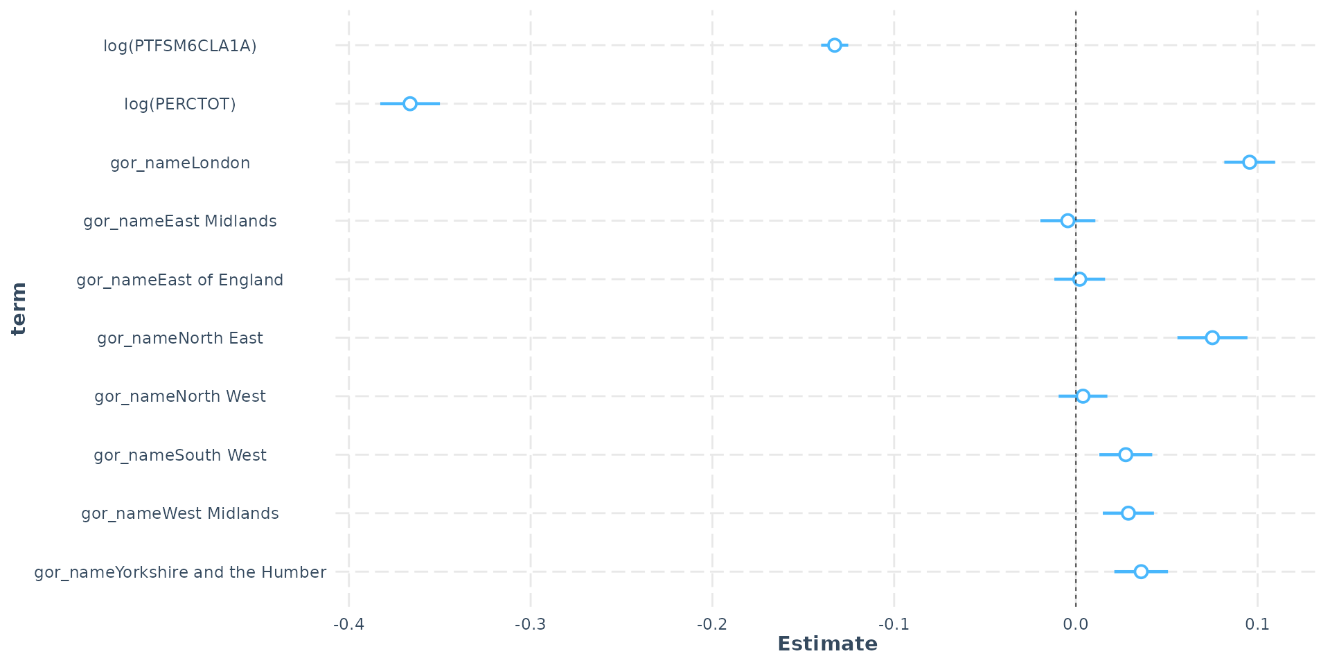
- There are 9 regions in England and here “London” has been set as the contrast or reference variable (which all others are compared to)
- Changing the contrast compares each region to a different reference
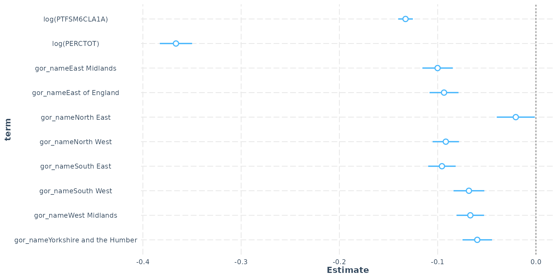
Dummy Variables
- Government Office Region (GOR) dummy - (London as ref)
Dummy Variables
Call:
lm(formula = log(ATT8SCR) ~ log(PTFSM6CLA1A) + log(PERCTOT) +
    gor_name, data = model_data)

Residuals:
     Min       1Q   Median       3Q      Max
-1.24928 -0.05827  0.00088  0.06062  0.73259

Coefficients:
                                  Estimate Std. Error t value Pr(>|t|)
(Intercept)                       5.014493   0.015398 325.660  < 2e-16 ***
log(PTFSM6CLA1A)                 -0.132708   0.003801 -34.910  < 2e-16 ***
log(PERCTOT)                     -0.366326   0.008373 -43.752  < 2e-16 ***
gor_nameLondon                    0.095655   0.007131  13.413  < 2e-16 ***
gor_nameEast Midlands            -0.004422   0.007724  -0.573 0.566995
gor_nameEast of England           0.002114   0.007119   0.297 0.766538
gor_nameNorth East                0.075134   0.009836   7.638 2.88e-14 ***
gor_nameNorth West                0.003926   0.006840   0.574 0.566020
gor_nameSouth West                0.027455   0.007428   3.696 0.000223 ***
gor_nameWest Midlands             0.028893   0.007181   4.023 5.87e-05 ***
gor_nameYorkshire and the Humber  0.035935   0.007533   4.770 1.92e-06 ***
---
Signif. codes:  0 '***' 0.001 '**' 0.01 '*' 0.05 '.' 0.1 ' ' 1

Residual standard error: 0.1025 on 3222 degrees of freedom
Multiple R-squared:  0.7182,    Adjusted R-squared:  0.7173
F-statistic:   821 on 10 and 3222 DF,  p-value: < 2.2e-16
- South East as contrast - London’s log(ATT8SCR) is 0.09 higher
- This equals (exp(0.095655) - 1) * 100 = 10% - London’s average Attainment 8 is 10% higher than the South East
Dummy Variables
- Hard to tell definitively from visual map, but residuals have changed and less clustering (Moran’s I would be more definitive - see GIS course)
Dummy Variables
- There is no correct contrast to choose for your dummy variable, you may need to try different ones to see which makes most intuitive sense
- Depending on the contrast, some dummy regions may or may not be statistically significant in comparison
- The inclusion of a regional dummy in this model has improved the \(R^2\) to 72%
- However, you may have noticed some of the coefficients have changed and this brings us to confounding and mediation
Variable Reclassification
A Quick Aside:
- One potentially useful strategy in regression modelling is the reclassification of an independent variable.
- Continuous -> Categorical or Weak Ordinal (e.g. various measurements of height into short, average and tall at different thresholds)
- Categorical -> Categorical with fewer categories (e.g. short, average, tall into below average and above average)
Variable Reclassification
- Benefits of reclassification:
- Moving from a continuous variable to a weak ordinal variable might make the patterns or observations easier to explain
- complex relationships (such as log-linear elasticities associated with absence from school) reduced to something more interpretable (if you miss more than 50% of school, your odds of passing your exams are drastically reduced)
- Previous obscured patterns can emerge from the data
- Collapsing categorical variables (e.g. multiple religious school denominations into religious/non-religious) can aid interpretability and boost statistical power, increase degrees of freedom
Variable Reclassification
- Risks of reclassification:
- Loss of statistical power due to loss of information
- Not always obvious where to make the cut when reclassifying a continuous variable and this can be crucial to the interpretation (e.g. is Low <20 or <30?)
Confounding
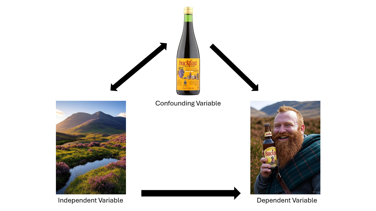
Confound: “to fail to discern differences between : mix up”
Confounding
![]()
Confounding
![]()
Confounding
- Confounding is the change in the effect on the dependent variable of the independent variables in the presence of each other
- Can occur when we know some independent variables might effect each other (such as disadvantage on absence) even when their joint presence doesn’t cause variance issues
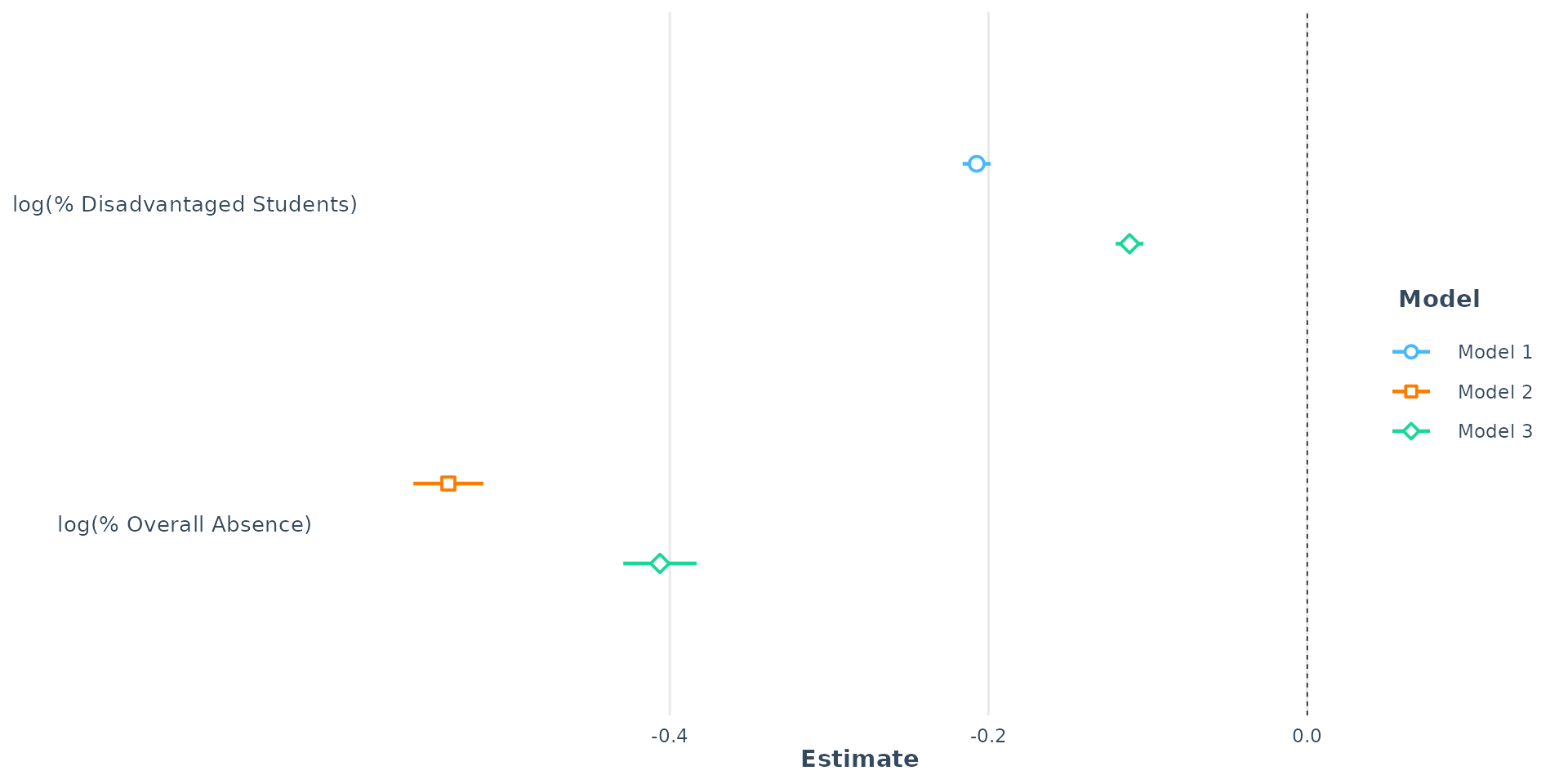
- Looking for confounding effects is a crucial part of model building - how do the coefficients of your model change when you introduce other variables?
Confounding
| 4.48 *** | 5.01 *** | 5.06 *** |
| -0.21 *** | | -0.11 *** |
| | -0.54 *** | -0.41 *** |
| 3248 | 3233 | 3233 |
| 0.45 | 0.60 | 0.69 |
- In the presence of Overall Absence, the effect of disadvantage is confounded (and vice versa)
- Both variables together, however, explain much more variation in Attainment 8 - both part of the story
Confounding
- The coefficient for log(PTFSM6CLA1A) - disadvantage - shrinks dramatically, from -0.21 down to -0.11 (a 44.5% reduction in effect)
- While the coefficient for log(PERCTOT) - Overall Absence - also shrinks from -0.54 to -0.41 this is just a 24.6% reduction
- The confounding effect of Overall Absence on disadvantage is almost double the confounding effect of disadvantage on Overall Absence
- This means that the relationship between disadvantage and Attainment 8 is much more biased by the omission of overall absence from the model than the other way around
Confounding
Call:
lm(formula = log(ATT8SCR) ~ log(PTFSM6CLA1A) + log(PERCTOT) +
    gor_name, data = model_data)

Residuals:
     Min       1Q   Median       3Q      Max
-1.24928 -0.05827  0.00088  0.06062  0.73259

Coefficients:
                                  Estimate Std. Error t value Pr(>|t|)
(Intercept)                       5.014493   0.015398 325.660  < 2e-16 ***
log(PTFSM6CLA1A)                 -0.132708   0.003801 -34.910  < 2e-16 ***
log(PERCTOT)                     -0.366326   0.008373 -43.752  < 2e-16 ***
gor_nameLondon                    0.095655   0.007131  13.413  < 2e-16 ***
gor_nameEast Midlands            -0.004422   0.007724  -0.573 0.566995
gor_nameEast of England           0.002114   0.007119   0.297 0.766538
gor_nameNorth East                0.075134   0.009836   7.638 2.88e-14 ***
gor_nameNorth West                0.003926   0.006840   0.574 0.566020
gor_nameSouth West                0.027455   0.007428   3.696 0.000223 ***
gor_nameWest Midlands             0.028893   0.007181   4.023 5.87e-05 ***
gor_nameYorkshire and the Humber  0.035935   0.007533   4.770 1.92e-06 ***
---
Signif. codes:  0 '***' 0.001 '**' 0.01 '*' 0.05 '.' 0.1 ' ' 1

Residual standard error: 0.1025 on 3222 degrees of freedom
Multiple R-squared:  0.7182,    Adjusted R-squared:  0.7173
F-statistic:   821 on 10 and 3222 DF,  p-value: < 2.2e-16
- Including a regional dummy slightly reduces the effect of Overall Absence and slightly increases the effect of disadvantage, relative to model 3
Confounding
Interpretation:
- Part of the negative effect of disadvantage was being suppressed or masked by the regional differences (probably London where Attainment 8 is higher on average and so are levels of disadvantage)
- Part of the negative effect of Overall Absence is due to its correlation with regional factors - but which ones?
- We can explore this question through one final twist in our modelling recipe - we can look at the interaction effects between individual regions and disadvantage / Overall Absence
Interaction Effects
- Put simply, an interaction term allows the model to answer the question: “Does the effect of disadvantage/Overall Absence on a school’s Attainment 8 score change from region to region?”
- Operationally, running interactions in the model simply requires variables to be multiplied together rather than summed
- Practically, the combinations of variables need some careful attention (or the assistance of a helpful Artificial Intelligence helper) to interpret correctly!
Interaction Effects
The equation for a model where we interact Overall Absence with Regions would look like:
\[\log(\text{Attainment8}) = \beta_0 + \beta_1 \log(\text{PctPersistentAbsence}) +\\\\ \sum_{j=1}^{k} \gamma_j \text{Region}_j + \sum_{j=1}^{k} \delta_j (\log(\text{PctPersistentAbsence}) \times \text{Region}_j) + \epsilon\]
Interaction Effects
Where (if we set the South East as the reference dummy)
- \(\beta_0\) is the intercept (predicted \(\log(\text{ATT8SCR})\) for the South East when - \(\log(\text{PERCTOT})=0\)).
- \(\beta_1\) is the main effect of unauthorised absence (the effect for the South East).
- \(\gamma_j\) is the difference in overall attainment for region \(j\) compared to the South East.
- \(\delta_j\) is the difference in the slope (effect of absence) for region \(j\) compared to the South East.
- \(\epsilon\) is the error term.
Interaction Effects
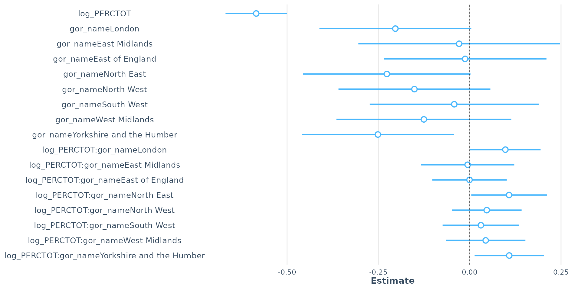
- 1% increase in the overall absence rate (log(PERCTOT)) predicts a 0.58% decrease in Attainment 8
- Controlling for overall absence, all other regions worse attainment than SE (reference). SE uniquely sensitive to absence
- Interaction effect: in London, NE & Yorkshire strong positive coefficient = negative effect of overall absence on attainment is significantly less severe than in SE
Interaction Effects
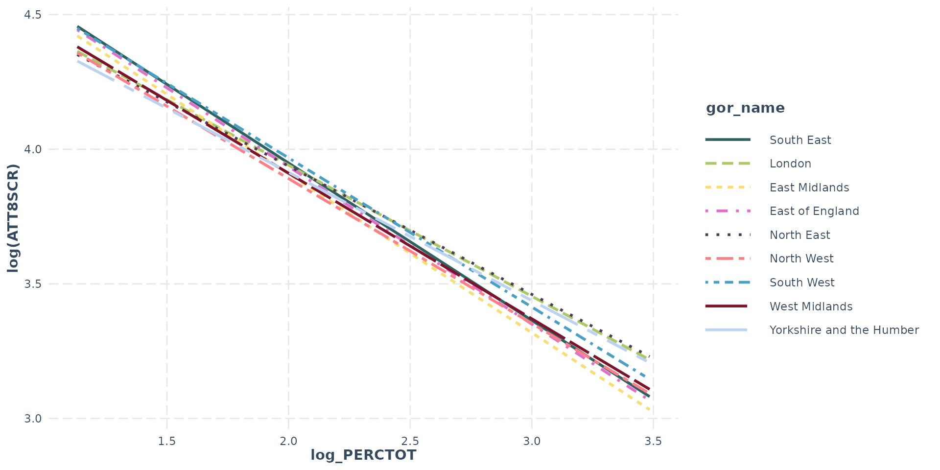
- Interacting disadvantage with region shows negative effect of disadvantage not as bad in regions other than SE - however…
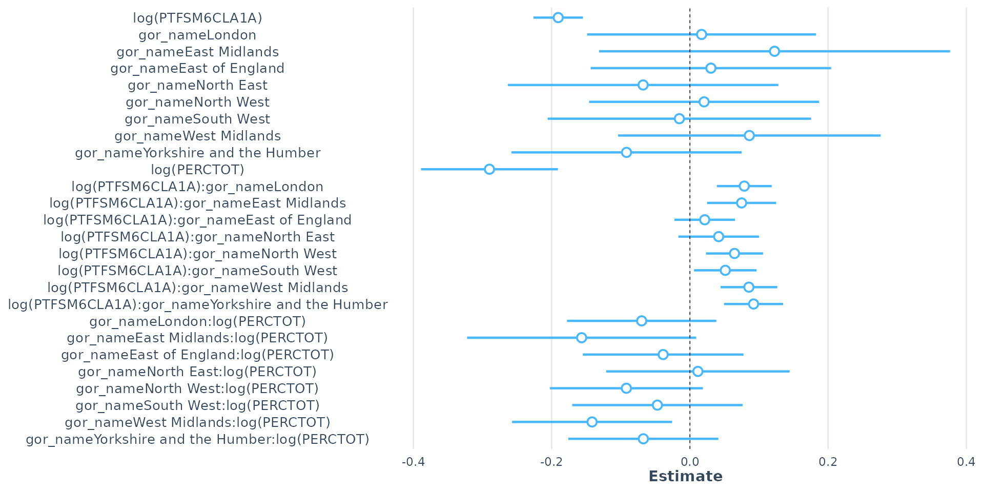
Interaction Effects
- As overall absence confounds disadvantage, so interacting both with region changes these effects
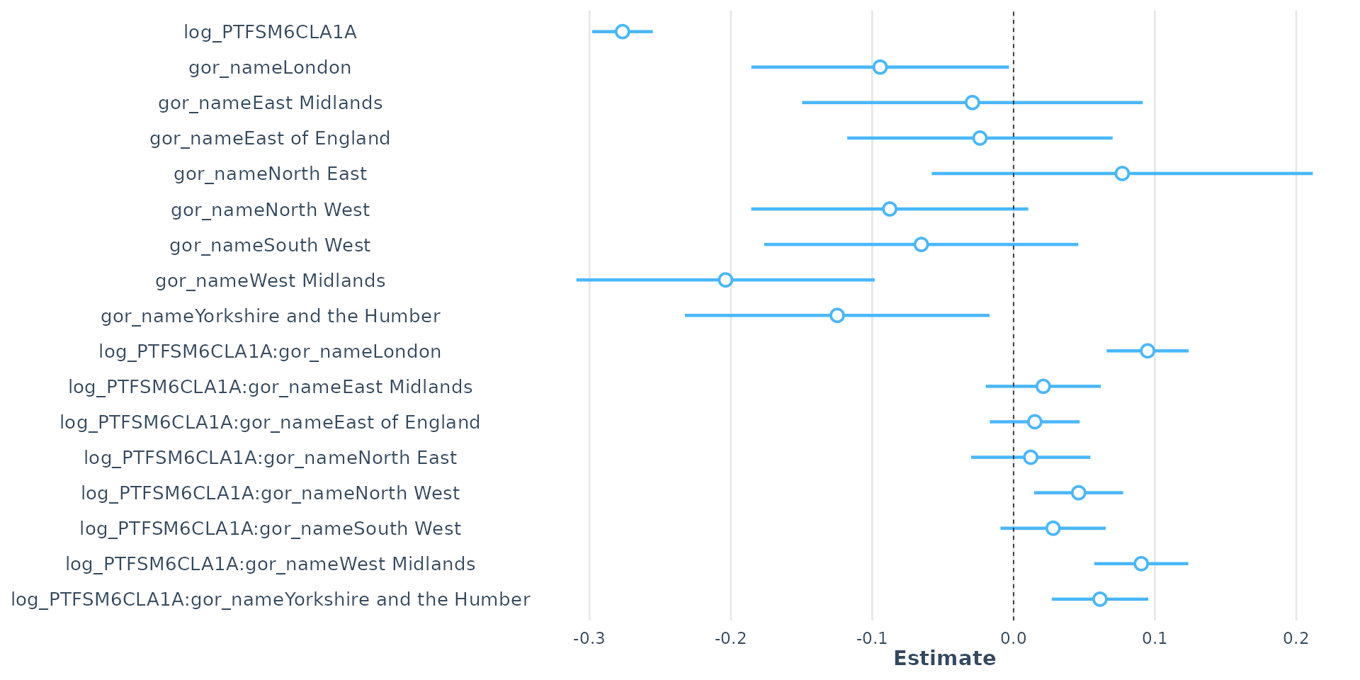
Interaction Effects
- Main Effect (Reference Group):
- The coefficient for log(PTFSM6CLA1A) is -0.190520. This is the effect of disadvantage in the South East.
- The coefficient for log(PERCTOT) is -0.289960. This is the effect of Overall Absence in the South East.
- Even when controlling for regional differences, unauthorised absence has a stronger negative effect on Attainment 8 than disadvantage
Interaction Effects
- Interaction Effects (Reference Group value + Other Region coefficient):
- log(PTFSM6CLA1A):gor_nameLondon: significant positive coefficient (+0.078684) - negative effect of disadvantage is less severe in London than in the South East
- same for all other regions - disadvantage has a more severe impact in the SE than anywhere else in England. SE schools particularly bad at mitigating effects of disadvantage
Interaction Effects
- Interaction Effects (Reference Group value + Other Region coefficient):
- gor_nameLondon:log(PERCTOT): The significant negative coefficient (-0.069792) - negative effect of Overall Absence is more severe in London than in the South East
- same for most other regions - Overall Absence as less severe impact in SE than anywhere else in England.
Interaction Effects
Call:
lm(formula = log(ATT8SCR) ~ log(PTFSM6CLA1A) * log(PERCTOT) +
    gor_name, data = model_data)

Residuals:
     Min       1Q   Median       3Q      Max
-1.24743 -0.05845  0.00082  0.06076  0.72702

Coefficients:
                                  Estimate Std. Error t value Pr(>|t|)
(Intercept)                       4.989742   0.064333  77.561  < 2e-16 ***
log(PTFSM6CLA1A)                 -0.125059   0.019674  -6.357 2.35e-10 ***
log(PERCTOT)                     -0.353934   0.032374 -10.933  < 2e-16 ***
gor_nameLondon                    0.095751   0.007137  13.417  < 2e-16 ***
gor_nameEast Midlands            -0.004420   0.007725  -0.572 0.567250
gor_nameEast of England           0.002028   0.007123   0.285 0.775845
gor_nameNorth East                0.075416   0.009864   7.646 2.72e-14 ***
gor_nameNorth West                0.004092   0.006853   0.597 0.550493
gor_nameSouth West                0.027349   0.007434   3.679 0.000238 ***
gor_nameWest Midlands             0.028953   0.007184   4.030 5.70e-05 ***
gor_nameYorkshire and the Humber  0.036074   0.007542   4.783 1.80e-06 ***
log(PTFSM6CLA1A):log(PERCTOT)    -0.003798   0.009586  -0.396 0.691945
---
Signif. codes:  0 '***' 0.001 '**' 0.01 '*' 0.05 '.' 0.1 ' ' 1

Residual standard error: 0.1025 on 3221 degrees of freedom
Multiple R-squared:  0.7182,    Adjusted R-squared:  0.7172
F-statistic: 746.2 on 11 and 3221 DF,  p-value: < 2.2e-16
- It is also possible to interact our continuous variables. However…
Interaction Effects
- Interaction term is statistically insignificant
- There is no evidence that the effect of concentrations of disadvantage on attainment changes based on the levels of unauthorised absence, or vice-versa
- Negative impact of disadvantage is roughly the same whether a school has a low or high unauthorised absence rate, and the negative impact of unauthorised absence is roughly the same regardless of the level of disadvantage
- Good to experiment as informative, but this interaction term can be removed from the model
Interaction Effects
- Final Note: Adding interaction effects will seriously increase your VIF as you are multiplying variables that are already in the model
- High VIF in a model with interaction terms does not affect the overall model.
- High VIF could inflate the standard errors of the coefficients making some otherwise significant variables seem insignificant
- Mean-Centring is a technique that could fix this, but we won’t look at it today
Interaction Effects
- Interpreting interaction effects is HARD (as you can probably tell from me trying to explain these!)
- AI is incredibly adept at interpreting outputs from regression models and describing the outputs in plain English. ChatGPT, Google Gemini, Claude and various others can be of great help here
- It doesn’t always get it right - never just feed an AI your outputs and trust its interpretation without questioning what it’s telling you
- Used correctly, however - particularly if you give it context with the data you are using and the patterns you are observing, it’s a tool that can really assist your understanding.
Some final thoughts on building regression models
- Aim is to try and explain as much variation in dependent variable as possible with the fewest number of independent variables
- More variables isn’t necessarily better - statistically insignificant variables might be worth dropping from your model
- As you add more variables, confounding might change the interpretation of earlier variables and may even stop them being statistically significant
- Algorithms like the Step-Wise algorithm can automate the process of variable selection - worth experimenting with, but no substitute for doing your own research!
- Building a good model takes time, experimentation, iteration and a lot of care and attention
Bringing it all together - our final regression show-stopper!
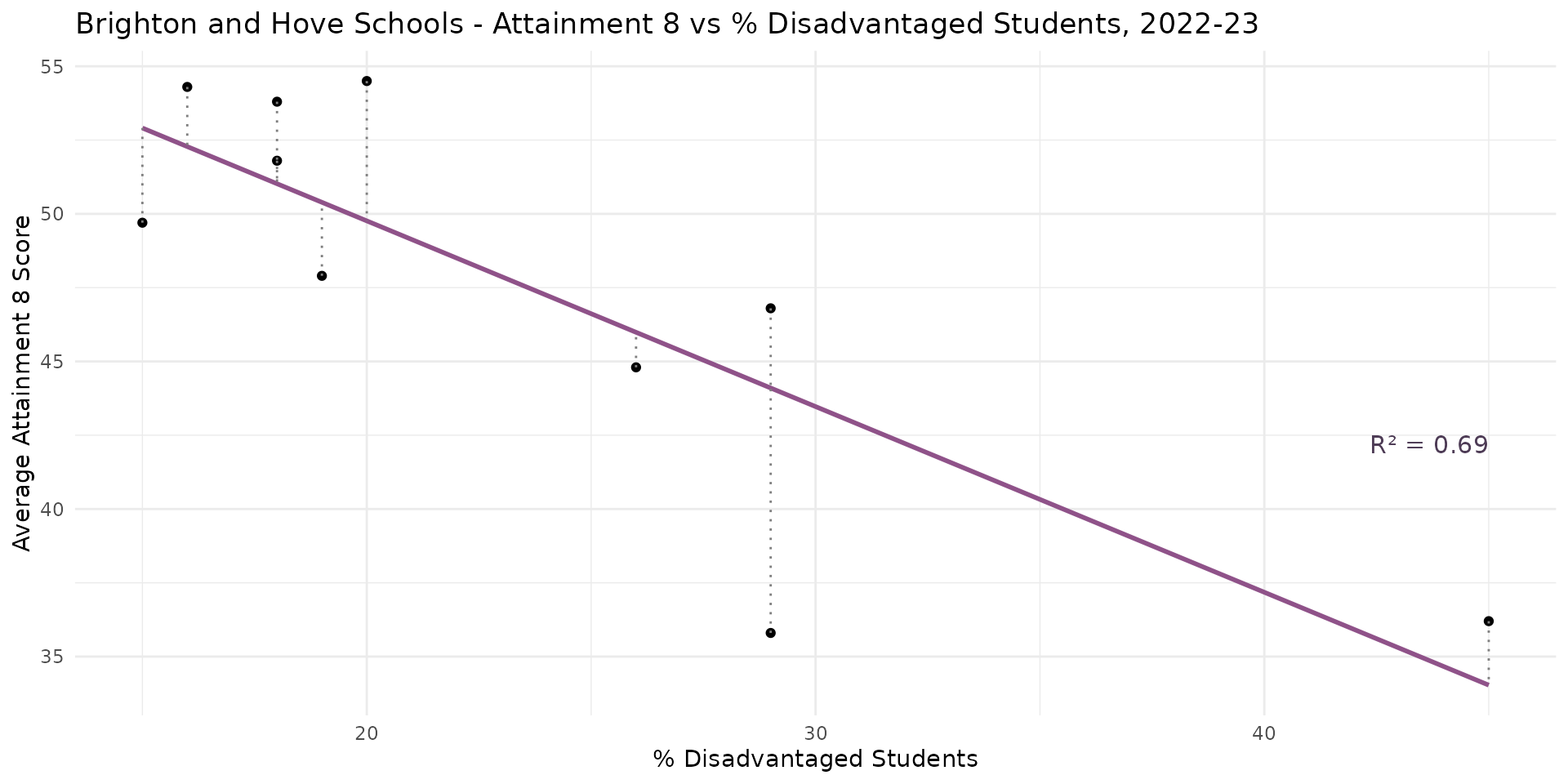
- In carefully building our regression model step-by-step, we have evolved our understanding:
- from a basic model for Brighton where it appeared that the % disadvantaged students in a school explained around 65% of the variation in Attainment 8 scores and a 10% decrease in disadvantage equating to a 6-point increase in Attainment 8
- to understanding that this initial local model was poor:
- few degrees of freedom
- unobserved confounding and mediation
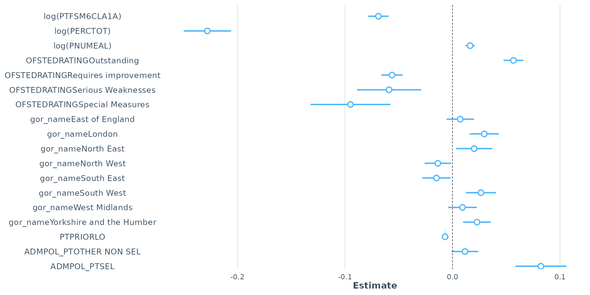
Bringing it all together - our final regression show-stopper!
Bringing it all together - our final regression show-stopper!
- Additional variables (some discussed, so not discussed in this lecture) have allowed us to explain almost 85% of the variation in Attainment 8 at the school level across England
- Careful interrogation of the coefficients as we have successively built up the complexity of the model reveals how the variables interact with each other
- The influence of disadvantage is partially confounded by overall absence
- but overall absence is a mediating variable in the relationship between disadvantage and attainment
Bringing it all together - our final regression show-stopper!
- Dummy variables can be your friend and allow us to compare how different groups perform in the data
- Ineracting variables can add even more explanatory power, but will take effort to interpret - AI can be your friend here if you are struggling
- If you follow the recipe, check you regression diagnostics at each stage and continually VISUALISE your data as you go, a good multiple regression model can be one of the most powerful explanatory tools in your toolbox!
This week’s practical
- Recreating much of what you have seen in this lecture yourself!
- Extending last week’s model and interpreting the outputs in Python or R
- This is another long practical - you won’t complete it in class today, so you should spend time at home (while listening to the Progression Sessions, preferably) working through this at your own pace.
- It is important that you are able to build your best model before next week’s lecture and practical session!