Linear Algebra
- beatrice.taylor@ucl.ac.uk
22nd October 2025
Maths underpins it

Image credit: [xkcd](https://xkcd.com/1838/)- This lecture covers some of the key concepts
- The goal is to facilitate deeper understanding of the methods
Maths doesn’t bite!
But what does it mean???
Equations are often used in the methods sections of papers to describe the model.
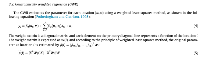
Taken from: Chiou, Jou, & Yang, (2015). Factors affecting public transportation usage rate: Geographically weighted regression. Transportation Research Part A: Policy and Practice.Machine learning
A model which improves after data is taken into account.
- Many of these concepts are also integral to machine learning
- Really just a specific type of mathematical model
- The learning part is about automatically finding patterns
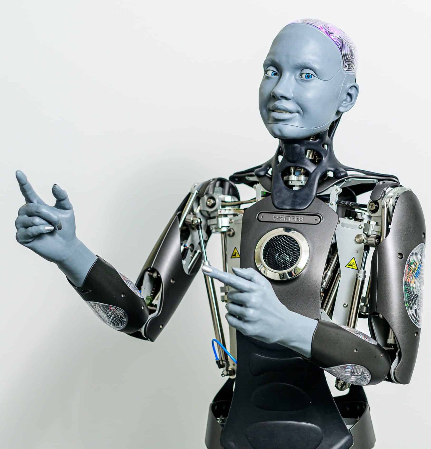
Embodied AI in the form of the creepy Ameca. Cheat sheet
Mathematical notation cheat sheet: https://www.upyesp.org/posts/makrdown-vscode-math-notation/

Numbers replaced by letters
The power to represent any number!
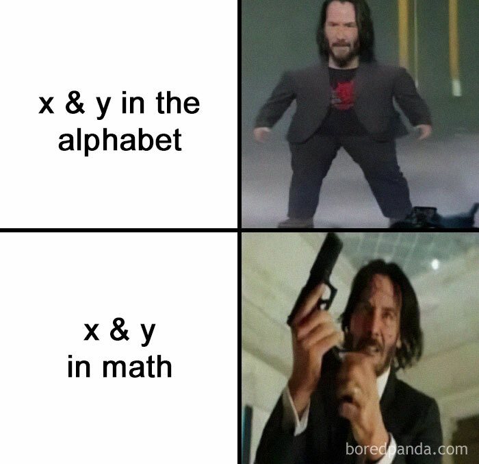
Keanu likes algebra. 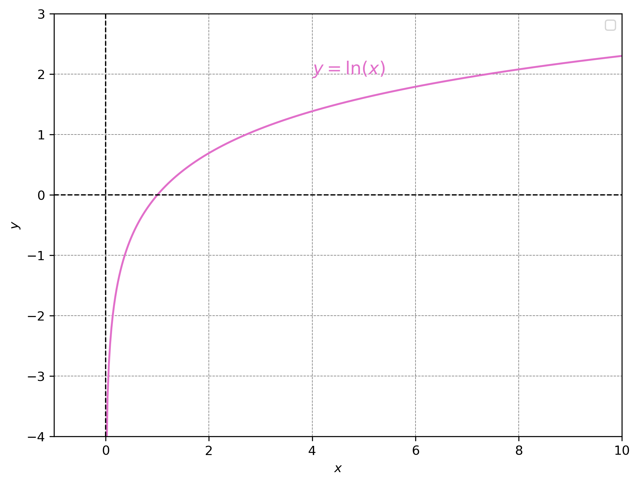
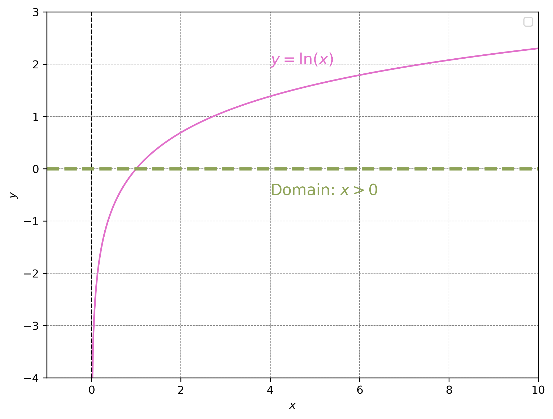
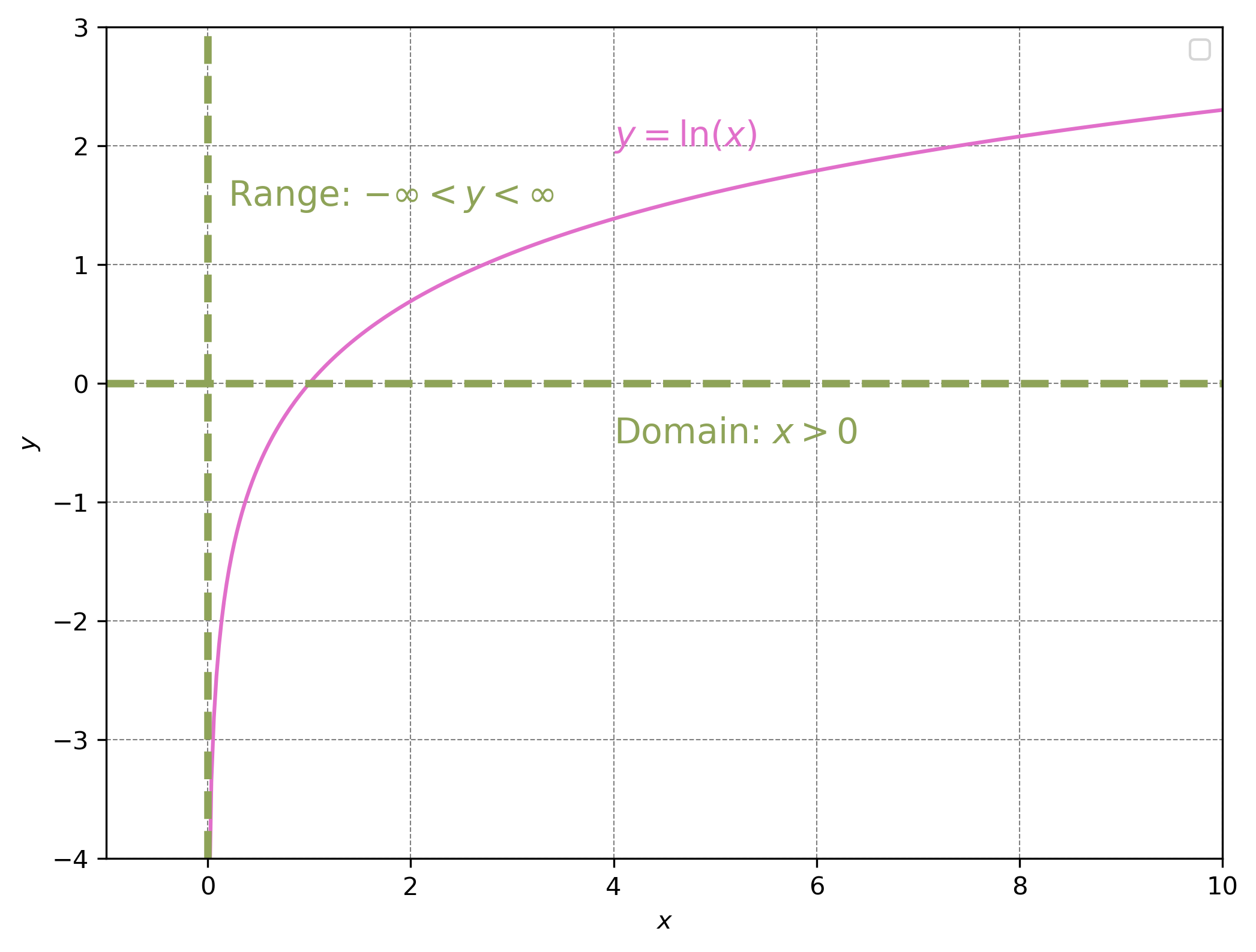
Question: what is the domain of \(ln(x)\)?
Question: what is the range of \(ln(x)\)?
Break

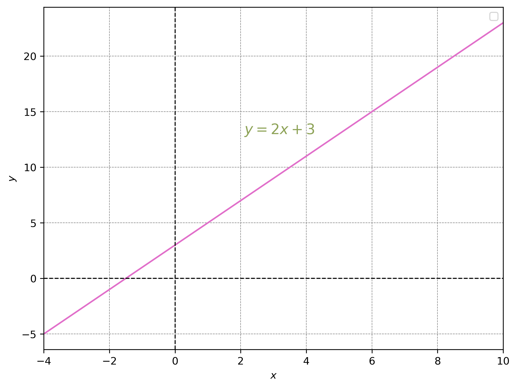
Straight lines
Graphically linear equations are straight lines.
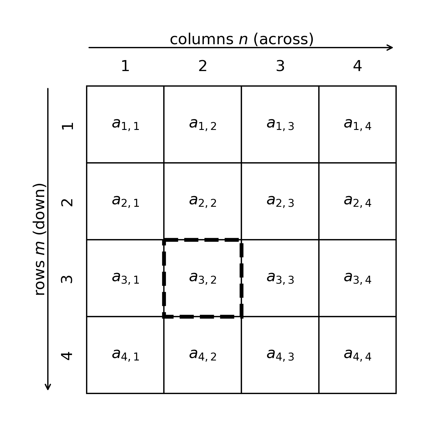
Down the stairs, along the corridor
Matrices are indexed by row (\(m\)) and by column (\(n\)).
So what does it mean?
Taken from: Chiou, Jou, & Yang, (2015). Factors affecting public transportation usage rate: Geographically weighted regression. Transportation Research Part A: Policy and Practice.Take another look
Chiou, Jou, & Yang, (2015). Factors affecting public transportation usage rate: Geographically weighted regression. Transportation Research Part A: Policy and Practice.

Covered

We’ve covered:
- Mathematical notation
- Sums and Products
- Functions
- Matrices
- Algebraic representations