Practical 3: Establishing and testing the hypothesis

This week is focussed on defining research hypotheses, and using statistical tests to evaluate them. In particular we will use the Student’s T-test, and the KS distribution test.

Note

This practical follows on from practical 2, so if you haven’t done that yet I suggest going back and working through that first!

Loading the data

We are going to look at schools perfomance data in England once again.

The data is sourced from and is downloadable here.

We have saved a copy of this dataset to the Github repo, in case that the dataset is removed from the website.

import pandas as pd
import matplotlib.pyplot as plt
import scipy.stats as sps
import numpy as np 

# Read CSV file, handling common missing value entries
na_vals = ["", "NA", "SUPP", "NP", "NE", "SP", "SN", "SUPPMAT"]
df_ks4 = pd.read_csv(
    'L2_data/england_ks4final.csv',
    na_values = na_vals
)

info_cols = ['RECTYPE', 'LEA', 'SCHNAME', 'TOTPUPS', 'TOWN']
ebaccs_cols = ['EBACCAPS', 'EBACCAPS_GIRLS', 'EBACCAPS_BOYS']

df = df_ks4[info_cols + ebaccs_cols]

df[['TOTPUPS']+ebaccs_cols] = df[['TOTPUPS']+ebaccs_cols].apply(pd.to_numeric, errors='coerce')

df = df[df['RECTYPE'].isin([1, 2])].copy()

df.head()

/tmp/ipykernel_12520/907340926.py:8: DtypeWarning:

Columns (75,77,78,79,80,81,82,83,84,85,86,87,88,89,90,91,92,93,94,144,145,146,147,148,149,150,151,152,177,178,179,180,181,182,183,186,187,188,189,190,191,192,194,195,196,198,199,200,202,203,204,206,207,208,210,211,212,214,215,216,218,219,220,222,223,224,230,233,234,235,236,237,238,239,242,243,244,245,246,247,248,251,252,253,254,255,256,257,266,267,268,269,270,271,272,281,282,283,284,285,286,287,296,297,298,299,300,301,302,311,312,313,314,315,316,317,335,336,337,340,341,342,345,346,347,366,367,368,369,370,371,372,373,374,375,376,377,378,379,380,381,382,383,384,385,386,387,388,389,390,391,392,393,394,395,396,397,398,399,400,401,402,403,404,405,406,407,408,409,410) have mixed types. Specify dtype option on import or set low_memory=False.

/tmp/ipykernel_12520/907340926.py:18: SettingWithCopyWarning:


A value is trying to be set on a copy of a slice from a DataFrame.
Try using .loc[row_indexer,col_indexer] = value instead

See the caveats in the documentation: https://pandas.pydata.org/pandas-docs/stable/user_guide/indexing.html#returning-a-view-versus-a-copy

	RECTYPE	LEA	SCHNAME	TOTPUPS	TOWN	EBACCAPS	EBACCAPS_GIRLS	EBACCAPS_BOYS
0	1	201.0	City of London School	1045.0	London	2.10	NaN	2.10
1	1	201.0	City of London School for Girls	739.0	London	1.51	1.51	NaN
2	1	201.0	David Game College	365.0	NaN	0.56	0.46	0.60
4	1	202.0	Acland Burghley School	1163.0	London	4.62	4.05	4.82
5	1	202.0	The Camden School for Girls	1047.0	London	6.25	6.25	NaN

Looking at the metadata (which you can see in ‘L2_data/ks4_meta.xlsx’) we can see the full meaning of each column header:

• ‘RECTYPE’ = Record type (1=mainstream school; 2=special school; 4=local authority; 5=National (all schools); 7=National (maintained schools))
• ‘LEA’ = Local authority
• ‘SCHNAME’ = School name
• ‘TOTPUPS’ = Number of pupils on roll (all ages)
• ‘TOWN’ = School town
• ‘EBACCAPS’ = Average EBacc APS score per pupil
• ‘EBACCAPS_GIRLS’ = Average EBacc APS score per girl
• ‘EBACCAPS_BOYS’ = Average EBacc APS score per boy

Research question

The department for education is worried about regional inequality in school grades. With this in mind they’ve come up with a research question they’d like to address.

Research question: Is average pupil attainment on the EBacc significantly different in London compared to the rest of England?

To do this we’re going to use the mean comparison test to compare the schools in London to those outside of London.

Preparing the data

Splitting the groups

For simplicity let’s create two dataframes for the two different areas.

df_London = df[df['TOWN'] == 'London']
df_London = df_London[df_London['EBACCAPS'].notna()]

df_notLondon = df[df['TOWN'] != 'London']
df_notLondon = df_notLondon[df_notLondon['EBACCAPS'].notna()]

And look at the summary statistics for each group.

df_London['EBACCAPS'].describe()

count    385.000000
mean       3.788260
std        1.851894
min        0.000000
25%        3.020000
50%        4.290000
75%        4.970000
max        8.700000
Name: EBACCAPS, dtype: float64

df_notLondon['EBACCAPS'].describe()

count    4246.000000
mean        3.395921
std         1.659090
min         0.000000
25%         2.820000
50%         3.670000
75%         4.380000
max         8.560000
Name: EBACCAPS, dtype: float64

From looking at the summary statistics the two groups are different sizes. The two groups also have different means - but we want to test if these means are statistically-significantly different.

The hypothesis test

We’re now going to work through the steps of the hypothesis test according to the five steps discussed in the lecture:

1. Define the null and alternative hypothesis
2. Set the significance level
3. Identify the evidence
4. Calculate the p-value
5. Compare p-value with hypothesis level

Step 1

What is the null and alternative hypothesis?

Question

H_0 = '??'
H_1 = '??'

print(f'The null hypothesis is {H_0}')
print(f'The alternative hypothesis is {H_1}')

Answer

H_0 = 'Mean EBacc score in London = Mean EBacc score outside London'
H_1 = 'Mean EBacc score in London > Mean EBacc score outside London OR Mean EBacc score in London < Mean EBacc score outside London'

print(f'The null hypothesis is {H_0}')
print(f'The alternative hypothesis is {H_1}')

The null hypothesis is Mean EBacc score in London = Mean EBacc score outside London
The alternative hypothesis is Mean EBacc score in London > Mean EBacc score outside London OR Mean EBacc score in London < Mean EBacc score outside London

Step 2

Set the significance level.

# Set the level of statistical significance 

alpha = 0.05

Step 3

Identify the evidence.

We already have the evidence - it’s our datasets df_London['EBACCAPS'] and df_notLondon['EBACCAPS'].

Step 4

Calculate the p-value.

We can use a built in function from scipy.stats called ttest_ind to do step 4 for us. You can read more about this function here.

First we need to check whether we can assume that the samples are drawn from populations with the same standard deviation or not. (Provided neither standard deviation is double the other, this should be ok).

London_std = df_London['EBACCAPS'].mean()
notLondon_std = df_notLondon['EBACCAPS'].mean()

# Calculate the ratio of standard deviations 
std_ratio = London_std/notLondon_std

print("std ratio =", std_ratio)

if std_ratio > 0.5 and std_ratio < 2:
    print("Can assume equal population standard deviations.")
    equal_stds = True
else:
    print("Cannot assume equal population standard deviations.")
    equal_stds = False

std ratio = 1.115532395766086
Can assume equal population standard deviations.

There are two outputs from the function scipy.stats.ttest_ind: the test statistic and the p value.

test_stat, p_value = sps.ttest_ind(df_London['EBACCAPS'], df_notLondon['EBACCAPS'], equal_var = equal_stds)

print("test statistic = ", test_stat)
print("p-value =", p_value)

test statistic =  4.398340904538903
p-value = 1.1153058452679495e-05

Step 5

Compare p-value with hypothesis level.

For the final step we compare the p-value to the significance value in order to reach a decision.

Question

if p_value ?? ?? :
    print(f"Reject the null hypothesis ({H_0}). Accept the alternative hypothesis ({H_1}).")
    print("Conclude that samples are drawn from populations with different means.")
elif p_value ?? ?? :
    print(f"No significant evidence to reject the null hypothesis ({H_0}).")
    print("Assume samples are drawn from populations with the same mean.")

Answer

if p_value < alpha:
    print(f"Reject the null hypothesis ({H_0}). Accept the alternative hypothesis ({H_1}).")
    print("Conclude that samples are drawn from populations with different means.")
elif p_value >= alpha:
    print(f"No significant evidence to reject the null hypothesis ({H_0}).")
    print("Assume samples are drawn from populations with the same mean.")

Reject the null hypothesis (Mean EBacc score in London = Mean EBacc score outside London). Accept the alternative hypothesis (Mean EBacc score in London > Mean EBacc score outside London OR Mean EBacc score in London < Mean EBacc score outside London).
Conclude that samples are drawn from populations with different means.

Hence we can conclude that the evidence supports there is a statistically significant differnece between the mean student attainment on the EBacc in London, versus outside of London.

A more complicated research question

Now I’d like to know, are the EBacc scores for boys and girls in England distributed similarly?

In the dataset we have the average EBacc score for each school split by gender. To address whether these two samples come from the same distribution we’re going to use the Kolmogorov-Smirnov two sample test.

Preparing the data

Summary statistics

As before, let’s start by looking at the summary statistics.

Question

df[[??]].??

Answer

df[['EBACCAPS_GIRLS', 'EBACCAPS_BOYS']].describe()

	EBACCAPS_GIRLS	EBACCAPS_BOYS
count	3851.000000	3801.000000
mean	3.820223	3.492636
std	1.409632	1.395525
min	0.000000	0.000000
25%	3.290000	2.980000
50%	3.950000	3.630000
75%	4.610000	4.250000
max	8.700000	8.560000

	EBACCAPS_GIRLS	EBACCAPS_BOYS
count	3851.000000	3801.000000
mean	3.820223	3.492636
std	1.409632	1.395525
min	0.000000	0.000000
25%	3.290000	2.980000
50%	3.950000	3.630000
75%	4.610000	4.250000
max	8.700000	8.560000

Plotting the data

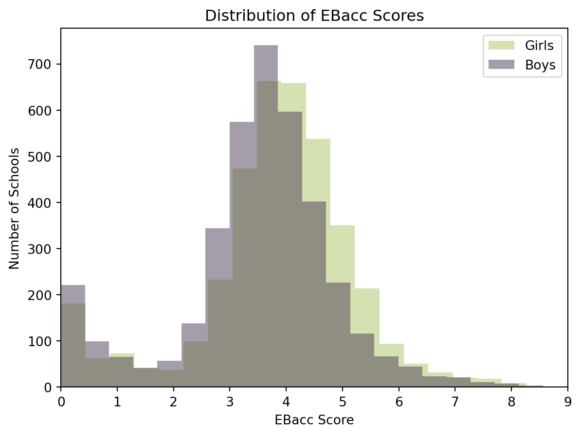
Let’s also visually inspect the data.

plt.hist(df['EBACCAPS_GIRLS'], bins=20, color='#abc766', alpha=0.5, label='Girls')
plt.hist(df['EBACCAPS_BOYS'], bins=20, color='#4e3c56', alpha=0.5, label='Boys')
plt.xlim(0,9) # the EBacc has a maximum score of 9
plt.xlabel('EBacc Score')
plt.ylabel('Number of Schools')
plt.title('Distribution of EBacc Scores')
plt.legend()

plt.show()

From visually looking at the plot we can see that the two distributions look quite similar - but we want to formally test that. As before, we’re going to follow the five steps of hypothesis testing.

Step 1

What is the null and alternative hypothesis?

Question

H_0 = '??'
H_1 = '??'

print(f'The null hypothesis is {H_0}')
print(f'The alternative hypothesis is {H_1}')

Answer

H_0 = 'Mean EBacc score for Girls is drawn from the same distribution as the mean EBacc score for Boys.'
H_1 = 'Mean EBacc score for Girls is drawn from a different distirbution to the mean EBacc score for Boys.'

print(f'The null hypothesis is {H_0}')
print(f'The alternative hypothesis is {H_1}')

The null hypothesis is Mean EBacc score for Girls is drawn from the same distribution as the mean EBacc score for Boys.
The alternative hypothesis is Mean EBacc score for Girls is drawn from a different distirbution to the mean EBacc score for Boys.

Step 2

Set the significance level.

Question

# Set the level of statistical significance 

alpha = ??

Answer

# Set the level of statistical significance 

alpha = 0.05

Step 3

Identify the evidence.

We already have the evidence - it’s our datasets df['EBACCAPS_GIRLS'] and df['EBACCAPS_BOYS'].

Step 4

Calculate the p-value

We can use a built in function from scipy.stats called ks_2samp to do step 4 for us. You can read more about this function here.

There are two outputs from the function scipy.stats.ks_2samp: the test statistic and the p value.

Question

ks_stat, ks_p_value = ?? 

print("KS test statistic = ", ks_stat)
print("KS p-value =", ks_p_value)

Answer

ks_stat, ks_p_value = sps.ks_2samp(df['EBACCAPS_GIRLS'].notna(), df['EBACCAPS_BOYS'].notna()) 

print("KS test statistic = ", ks_stat)
print("KS p-value =", ks_p_value)

KS test statistic =  0.0088386070355312
KS p-value = 0.9799658737017607

Step 5

Compare p-value with hypothesis level.

For the final step we compare the p-value to the significance value in order to reach a decision.

Question

if ??
    print(??)
else ?? 
    print(??)

Answer

if ks_p_value < alpha:
    print(f"Reject the null hypothesis that the samples are drawn from the same distribution.")
    print("Conclude that samples are drawn from populations with different distributions.")
else: 
    print(f"Fail to reject the null hypothesis that the samples are drawn from the same distribution.")
    print("Assume that samples are drawn from populations with the same distribution.")

Fail to reject the null hypothesis that the samples are drawn from the same distribution.
Assume that samples are drawn from populations with the same distribution.

Extension

If you’ve finished working through the examples in the tutorial then have a go at coming up with your own research question and hypothesis.

A good place to start would be by looking at the data in df_ks4 - theres a lot of numerical information here - are there two variables you could compare?

df_ks4.hist(bins=50, figsize=(20, 15))
plt.tight_layout()
plt.show()

You’re Done!

Well done you’ve completed this weeks practical on establishing and evaluating hypothesis questions. If you are still working on it, take your time. If you have any questions just ask!