Hypothesis Testing

Establishing and evaluating research hypotheses

Beatrice Taylor - beatrice.taylor@ucl.ac.uk

8th October 2025

Last week

Overview of lecture 2

Continued concepts from exploratory data analysis, in particular probability distributions.

• Representative data
• Normal distribution
• Binomial distribution
• Poisson distribution
• Exponentials
• Logarithms

This week

Motivation

How do we understand how likely events are to occur?

Question

What is the probability of someone at UCL being over 190cm?

Answer

Try to understand the distribution of heights.

Last week we asked this question and we thought about the distribution of the data. How to describe the distribution of the data mathematically.

This week we look at how to properly ask the research question, and how to answer it.

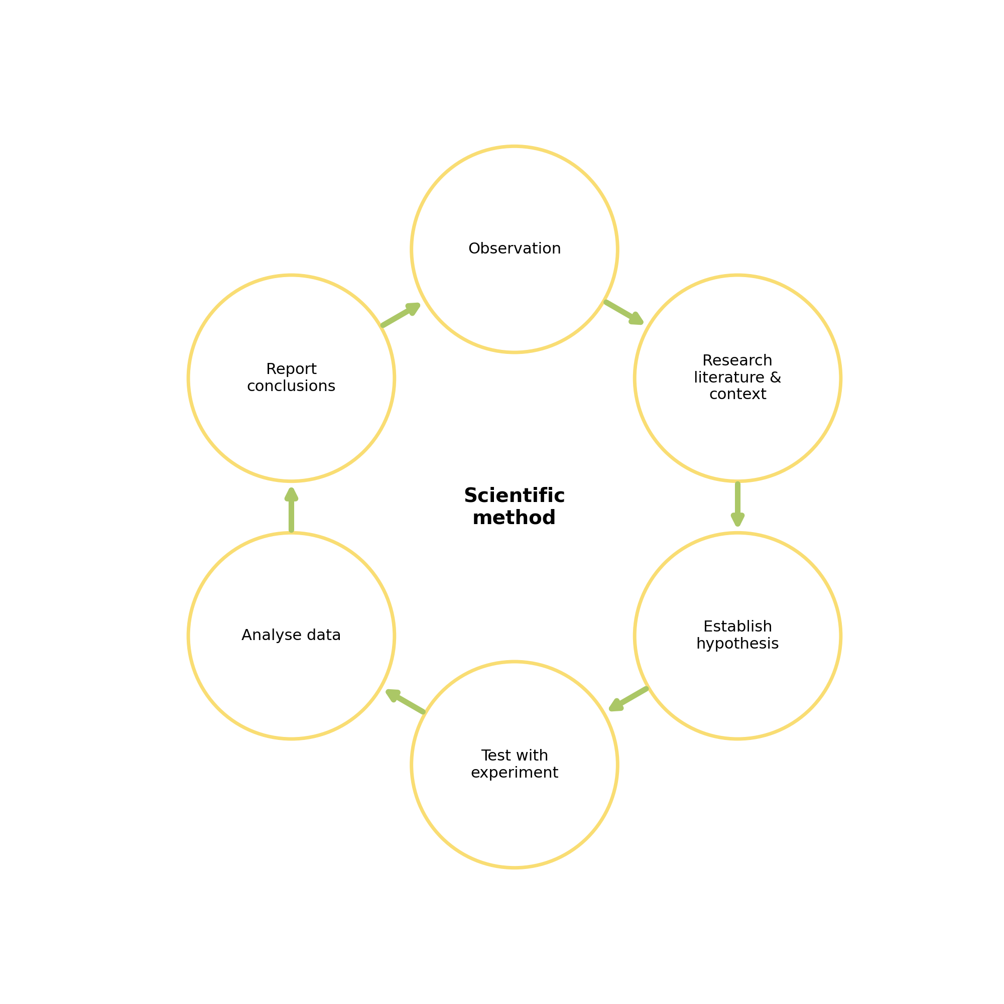
The scientific method

Statistical tests: - formal way to define a threshold of what is an interesting result - and hence evaluate the hypothesis

Last week we looked at exploratory data analysis - now the formal process of coming up with and evaluating questions - very much part of the scientific method.

Why is this important?

We see stories in the news, how do we know what to believe and what not to believe? This is where having an understanding of statistical tests can help us - we can evaluate claims to try and figure out which are/ aren’t statistically significant.

A clearly defined, and reproducible way to evaluate findings.

Learning Objectives

By the end of this lecture you should be able to:

1. Establish a hypothesis for a given research project.
2. Define the Type I and Type II errors.
3. Evaluate a hypothesis using appropriate statistical tests.

How do you come up with a hypothesis?

Research question vs. hypothesis

Research question

A research question focuses on a specific problem.

Hypothesis

A formal statement that you will seek to prove or disprove.

The hypothesis is a statement you can explicitly test. It can either be true or false - and hence using evidence you can come to a judgement about it’s truth value.

Flip a coin

• You have a coin.
• You think it’s a fair coin.
• You toss it 10 times.
• It comes up heads 7 times.

What do you think is the hypothesis here?

Ask the class.

Hint: which of these is something you can actually test?

The hypothesis

• You have a coin.
• You think it’s a fair coin.
• You toss it 10 times.
• It comes up heads 7 times.

The hypothesis is that it is a fair coin.

Question for the class - whats the evidence?

The 10 coin flips and the observation of 7 heads is the evidence

The evidence

• You have a coin.
• You think it’s a fair coin.
• You toss it 10 times.
• It comes up heads 7 times.

The observations are the evidence.

What question can you ask?

• You have a coin.
• You think it’s a fair coin.
• You toss it 10 times.
• It comes up heads 7 times.

Is it a fair coin?

What’s the probability that it’s fair?

If the coin is fair, how likely would it be to see 7 heads out of 10 flips?

All these questions are difficult to evaluate.

What question should you ask?

• You have a coin.
• You think it’s a fair coin.
• You toss it 10 times.
• It comes up heads 7 times.

Correct formulation:

If the coin is fair, how likely would it be to see 7 heads out of 10 flips or an even more extreme result?

Interested in the probability of seeing the event or something even more extreme.

Establishing and evaluating a hypothesis

In five simple steps.

Step 1

Define the null and alternative hypothesis

\(H_0\) - the null hypothesis

• this is the “status quo”
• it is assumed to be true

\(H_1\) - the alternative hypothesis

• your hypothesis
• it requires some evidence (i.e. data) to verify
• it directly contradicts the null hypothesis

Be careful in how the two are defined. Logically H_1 needs to directly contradict H_0.

For example if my H_0 was everyone likes chocolate. H_1 couldn’t be some people prefer biscuits - since in this situation both H_0 and H_1 can be true at the same time. H_1 would have to be that not everyone likes chocolate.

Step 2

Set your significance level \(\alpha\)

The significance level is the threshold below which you reject the null hypothesis.

• Decide what “too unlikely” means
• Common choice is 5% significance
  • \(\alpha = 0.05\)
  • This means that if we see evidence that would have less than a 5% chance of occurring under the null hypothesis, then we reject the null hypothesis.

WARNING

Decide what “too unlikely” means before you do the test

• otherwise considered ‘HARKing’
  • Hypothesising
  • After
  • the
  • Results
  • are
  • Known

It’s important to decide on your significance level prior, as otherwise you might find an event which is significant at the 10% threshold and not at 5% - which could lead to bad scientific practise.

There’s a balance - often we don’t know what will be interesting - so you do some exploratory data analysis. But you shouldn’t be fishing around for stuff - needs to be grounded in theory and literature.

Step 3

Identify the evidence

• This could mean collecting the data
• Or identifying a suitable existing dataset
  • Crucial that it’s suitable - think about biased/ unrepresentative data

In quant methods this normally means finding an open public dataset to use.

The evidence needs to be suitable to answer the question - think about biased/representative data from last week. Something they will be assessed on in the assessment.

Step 4

Calculate the p-value

The p-value is the probability of seeing the evidence, or something even more extreme, if the null hypothesis is true.

• Calculated according to the appropriate statistical test
• The choice of test is determined by the research question and the data

We’ll come back to different types of statistical test later in the lecture

Step 5

Compare p-value with significance level

• p-value \(> \alpha\)
  • Evidence not that unlikely.
  • Not enough evidence to reject \(H_0\).
• p-value \(\leq \alpha\)
  • Evidence very unlikely.
  • Reject \(H_0\) and accept \(H_1\).

The steps

In order to evaluate our hypothesis we just have to do the five steps:

1. Define the null and alternative hypothesis
2. Set you significance level
3. Identify the evidence
4. Calculate the p-value
5. Compare p-value with hypothesis level

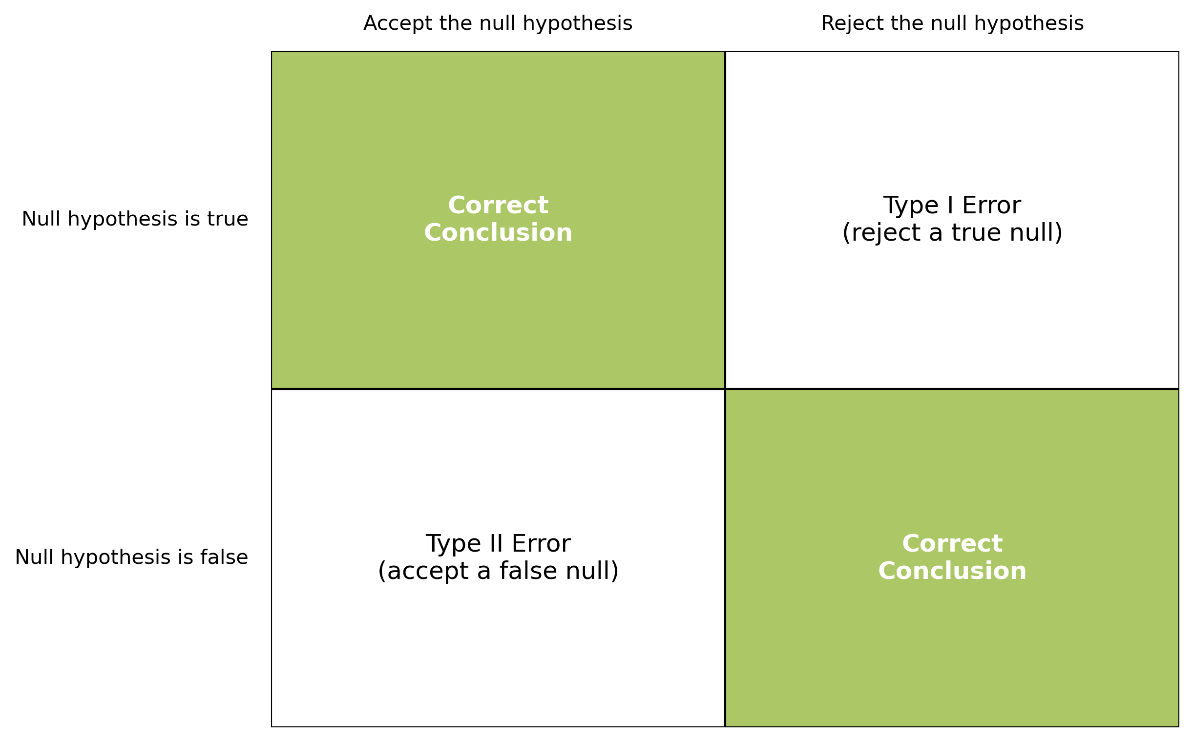
Types of error

… where things can go wrong.

Type I error

The true null hypothesis is incorrectly rejected.

The null hypothesis is true, but you get a false positive leading to you rejecting the null hypothesis.

This is also called a false positive.

Example: In court a defendant is found guilty despite being innocent.

Type II error

The false null hypothesis is incorrectly accepted.

The null hypothesis is false, but you get a false negative result, leading you to accepting the null hypothesis.

This is also called a false negative.

Example: In court a defendant is found innocent despite being guilty.

Example: Mammograms

NHS offers breast cancer screening for all people with breasts between the ages of 50 and 70.

The idea is to screen all those in the population who are at high risk of breast cancer - in the hope they pick up results better.

Whilst the tests are good they’re not 100% accurate.

Example: Screening outcomes

The hypothesis:

\(H_0:\) The individual doesn’t have breast cancer.

\(H_1:\) The individual does have breast cancer.

Example: Evaluating the evidence

From NHS digital.

Type I error: false positive

• In 2020-2021, 4.0% of those screened had an abnormal results and were referred for assessment.
• Of these, 77.1% were found to not have breast cancer at follow up assessment.
• Leading to a false positive rate of 3.1%.

This false positive rate is calculated as 4% times 77.1%

False positive is bad as you might pursue a healthcare treatment which is actually unecessary for the patient.

Example: Evaluating the evidence

From NHS digital.

Type II error: false negative

• Those who had a negative screening but did in fact have breast cancer.
• Harder to calculate the false negative rate, as they might be diagnosed with breast cancer at any later point in time.
• Studies suggest the false negative rate could be as high as 20%.

False negative - in healthcare context this is the worst outcome - as goes undiagnosed and hence untreated.

Matrix of errors

Possible outcomes form a matrix. Have two good outcomes, and two bad outcomes which we want to look out for (these are the Type I and Type II errors).

This is something to bear in mind when we look at evaluating our hypotheses. How good is our data, so how reliable is our outcome?

Often this language is used when evaluating the outcomes of an ML classification model. Where we report the quality of a supervised model in terms of its rate of false positives and false negatives.

A good hypothesis or a bad hypothesis?

Understanding the literature and the context

The hypothesis should not come out of thin air.

Should consider:

• What do you know about the context?
• What research have other people done?

Asking ethical hypothesis questions

It’s important to not make unethical assumptions in choosing the hypothesis.

Example

Police profiling - assumes a correlation between appearance and crime

• Use contextual knowledge
• Is this causation?
• Or correlation linked to other factors?

There is an assumption that theres a link between how someone looks and what crime they are likley to commit - leading to potentially racist police profiling - as assuming a link between ethnicity and likelihood to commit a crime.

Correlation vs. Causation

Correlation: Two variables are statistically related, as one changes so does the other.

Causation: One variable influences the other variable to occur.

Causation implies correlation.

BUT correlation does not imply causation!

Lots of things can be correlated BUT it doesn’t mean one event caused another.

Aliens and librarians

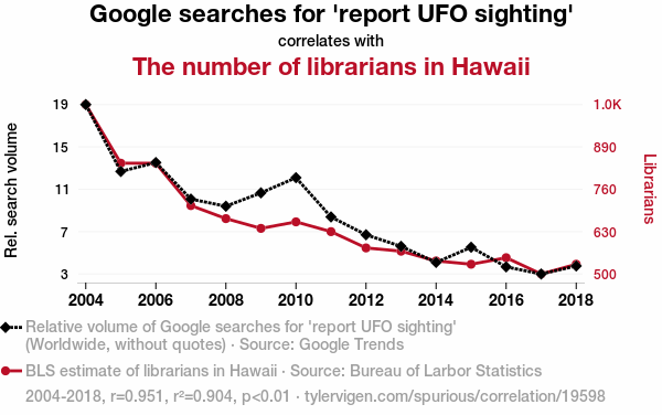
Image credit: [Spurious Correlations](https://www.tylervigen.com/spurious/correlation/19598_google-searches-for-report-ufo-sighting_correlates-with_the-number-of-librarians-in-hawaii)

It’s a dumb example but it’s quite easy to find nonsense correlations between random variables. Can generate your own at the website spurious correlations.

Correlation IS NOT causation

You might not know whether events are correlated, or causing each other

BUT

you should use your contextual understanding to come up with plausible (and ethical) initial questions.

Sometimes it’s hard to figure out if two variables are correlated or causational. There can be all sorts of complexities - like confounding factors, which can be hard to spot. The point is to do your best to come up with plausible and ethical intial questions.

And then the point of hypothesis testing is figuring out whether the evidence you have is siginificant enough to support you hypothesis.

Will return to looking at the mathematical correlation between variables in week 5.

The point of the scientific method

It’s a process

• question
• test
• evaluate
• REPEAT!

Returning to the idea of the scientific method is that it’s iterative.

Maybe we initially made the wrong assumptions but we can repeat, and update our ideas.

Example: students height

Research question
Are male and female students similar heights?

Research hypothesis
Male and female students are different heights on average.

Going to look at applying the five steps of hypothesis testing to a specific example.

Example - step 1

Define the null and alternative hypothesis

\(H_0\): The mean height of male and female students is the same.

\(H_1\): The mean height of male and female students is different.

Example - step 2

Set your significance level

\(\alpha = 0.05\)

Example - step 3

Identify the evidence

I’ve collected data from 198 students, as follows:

Group	Sample Size	Mean (cm)	std (cm)
Female students	95	170	5
Male students	103	180	6

Example - step 4

Calculate the p-value

Aha!

How do we do this? We need to know what statistical test to use!

Statistical tests

Numerically testing whether the data supports the hypothesis.

Parametric vs. Non-parametric tests

Parametric tests

• Assumptions about the distribution:
  • Normal distribution
  • Independent and unbiased samples
  • Equal/comparable variances
  • Continuous data

Non-parametric tests

• Typically less assumptions on the distribution
• Continuous or discrete data

Two main categories of test.

Deciding on a test

• It can be hard to figure out what test to use.
• Going to cover some common tests
• Might also find these useful:
  • flowchart
  • table

Sometimes its clear what test to use, but sometimes it’s not. All sorts of obscure statistical tests from different disciplines.

Focusing on a few tests which might be useful for the types of data we’re likely to come across.

Additional resources for identifying tests - typically based on flowchart of whether assumptions are met or not.

Parametric tests

Student’s T-test

Student’s T-test is used to compare the mean of a dataset.

• parametric statistical test
• assumes the data is normally distributed

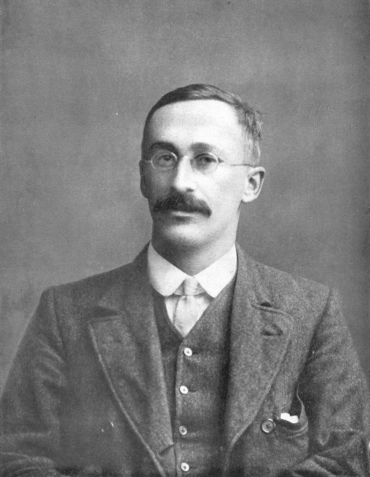
This is William Sealy Gosset - he was **not** a student.
Image credit: https://en.wikipedia.org/wiki/William_Sealy_Gosset#/media/File:William_Sealy_Gosset.jpg

William Gosset was working for Guinness brewing company when he came up with the t-test - but his company wanted his to publish under a pseudonym - hence ‘student’. He was comparing the chemical properties of different samples of barley.

Student’s T-test: steps

Calculate:

• test statistic (called the t value)
  • The test statistic is a number that summarises the data so as to determine whether to reject the null hypothesis.
• degrees of freedom
  • The number of degrees of freedom is the number of values in the final calculation that are free to vary.

Which we use to identify the p value - typically using a ‘look up table’.

Use the test statistic and the degrees of freedom to get the p-value. Might remember look up tables from maths at school - instead we’ll be using python.

Student’s T-test: types

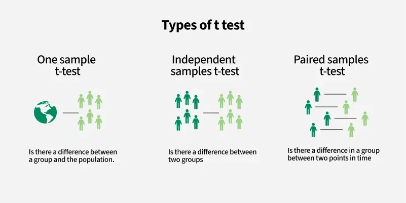
Image credit: https://www.geeksforgeeks.org/data-science/t-test/

3 main types of test depending on what we’re interested in.

Student’s T-test: one sample

Tests whether the population mean is equal to a specific value or not

The test statistic is calculated as:

\[\begin{align} t = \frac{\bar{x} - \mu_{0}}{s / \sqrt{n}} \end{align}\]

where

• \(\bar{x}\) is the sample mean
• \(\mu_{0}\) is the hypothesised population mean
• \(s\) is the sample standard deviation
• \(n\) is the sample size

Student’s T-test: one sample, degrees of freedom

The number of degrees of freedom is the number of values in the final calculation that are free to vary.

\[\begin{align} df = n-1 \end{align}\]

Student’s T-test: two sample

Tests if the population means for two different groups are equal or not.

The test statistic is:

\[\begin{align} t = \frac{\bar{x}_1 - \bar{x}_2}{s_p \sqrt{\frac{1}{n_1} + \frac{1}{n_2}}} \end{align}\]

• \(\bar{x}_1, \bar{x}_2\) are the sample means of groups 1 and 2
• \(n_1, n_2\) are the sample sizes of groups 1 and 2
• \(s_p\) is the pooled standard deviation

\[\begin{align} s_p = \sqrt{\frac{(n_1 - 1)s_1^2 + (n_2 - 1)s_2^2}{n_1 + n_2 - 2}} \end{align}\]

with \(s_1, s_2\) the sample standard deviations.

Student’s T-test: two sample, degrees of freedom

The number of degrees of freedom is the number of values in the final calculation that are free to vary.

In the two-sample Student’s T-test the degrees of freedom are:

\[\begin{align} df = n_1 + n_2 - 2 \end{align}\]

Student’s T-test: paired

Tests if the difference between paired measurements for a population is zero or not - normally used with longitudinal data.

The test statistic is:

\[\begin{align} t = \frac{\bar{d}}{s_d / \sqrt{n}} \end{align}\]

where

• \(\bar{d}\) is the mean of the paired differences
• \(s_d\) is the standard deviation of the paired differences
• \(n\) is the number of pairs
• the number of degress of freedom is \(n-1\)

For example used when I have data from different years, and want to figure out if there’s a difference across the years.

You need to be able to pair the data - i.e. the same things being observed at time point 1 and time point 2.

How many tails?

Tests can be one-tailed or two-tailed - which you want is determined when you define the hypothesis.

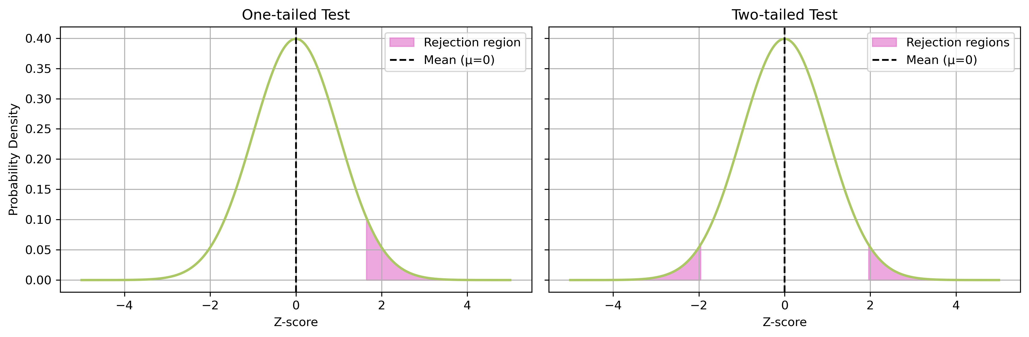
One tailed: if you only care is the mean is significant in one direction

Two tailed: if you care about the mean being different regardless of direction

Soemthing else to consider - this becomes relevant when we look up the p-value

Non-parametric tests

Kolmogorov-Smirnov

• Compares two probability distributions
• Can be used to test whether an observed sample came from a given distribution
• Or to test whether two samples both came from the same distribution

Named after two Russian soviet mathematicians working in the mid 20th century

K-S test: one sample test

Tests if a sample dataset came from a known distribution.

The Kolmogorov–Smirnov test statistic is:

\[\begin{align} D_n = \sup_x \, | F_n(x) - F(x) | \end{align}\]

where

• \(F_n(x)\) is the empirical distribution function (EDF) of the sample
• \(F(x)\) is the cumulative distribution function (CDF) of the reference distribution

Note

‘\(sup\)’ is the suprenum - think of it as the smallest upper bound.

‘sup’ is a maths - don’t need to know what it means - just intuitively its measuirng the smallest upper bound on the difference between the two distirbutions.

Thinking back to last week we might use the K-S test to determine if a dataset is drawn from a noraml distirbution by comapring to the normal cumulative distribution function.

K-S: empirical distribution function

The empirical distribution function (EDF) is:

\[\begin{align} F_{n}(x) = \frac{1}{n} \sum_{i=1}^{n} 1_{(-\infty ,x]}(X_{i}) \end{align}\]

where

• \(n\) is the number of observations
• \(X_i\) are the ordered sample values
• \(1_{(-\infty ,x]}(X_{i})\) is an indicator function (1 if \(X_i \leq x\), else 0)

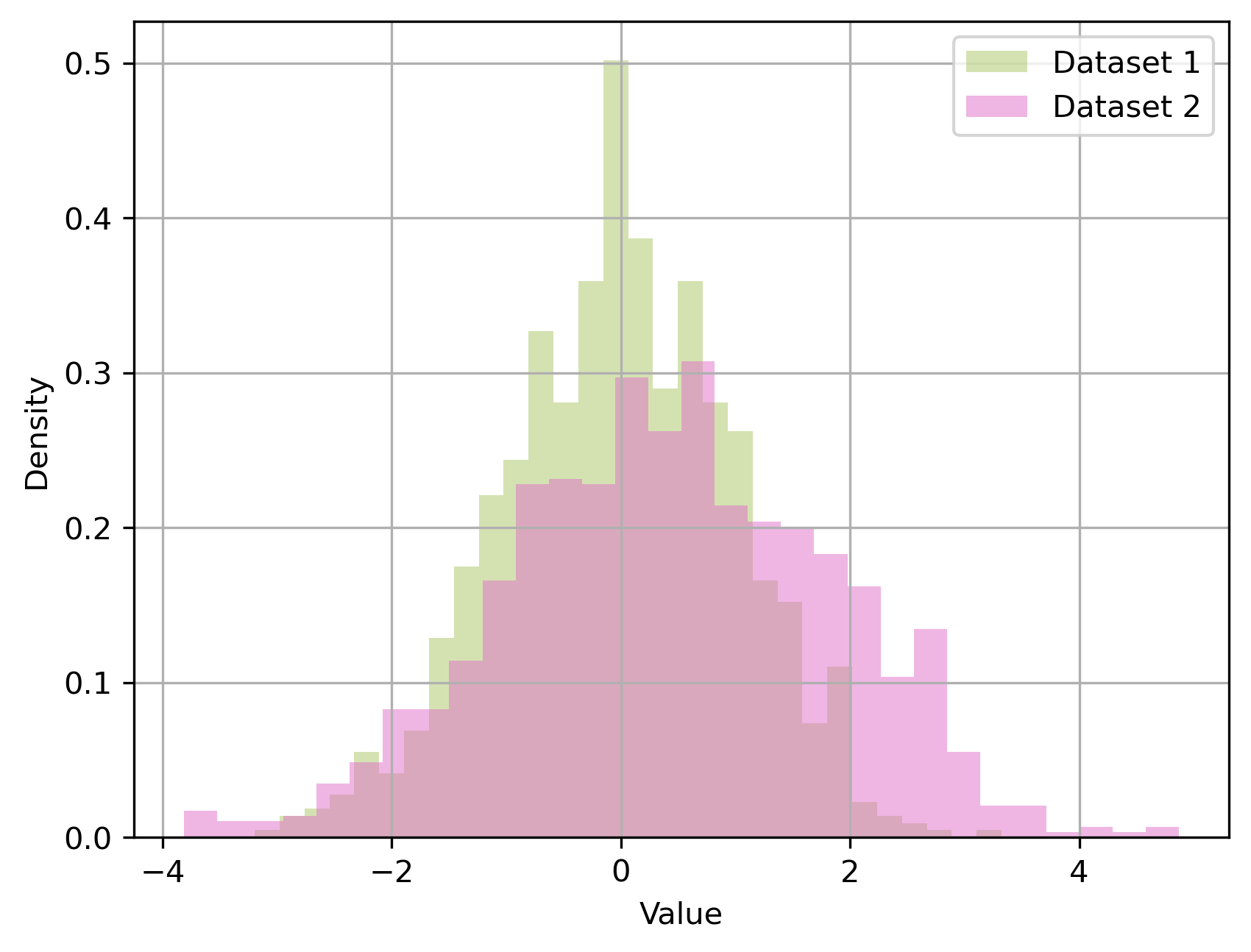
K-S test: two sample test

Tests if the underlying distributions of two sample datasets are the same.

For the two-sample test:

\[\begin{align} D_{n,m} = \sup_x \, | F_n(x) - G_m(x) | \end{align}\]

where

• \(F_n(x)\) and \(G_m(x)\) are the EDFs of the two samples.

K-S test: decision rule

The hypotheses would be:

• \(H_0\): the distributions are the same
• \(H_1\): the distributions differ

Larger values of the test statistic \(D\) is stronger evidence against \(H_0\).

How do we use the K-S test is practise?

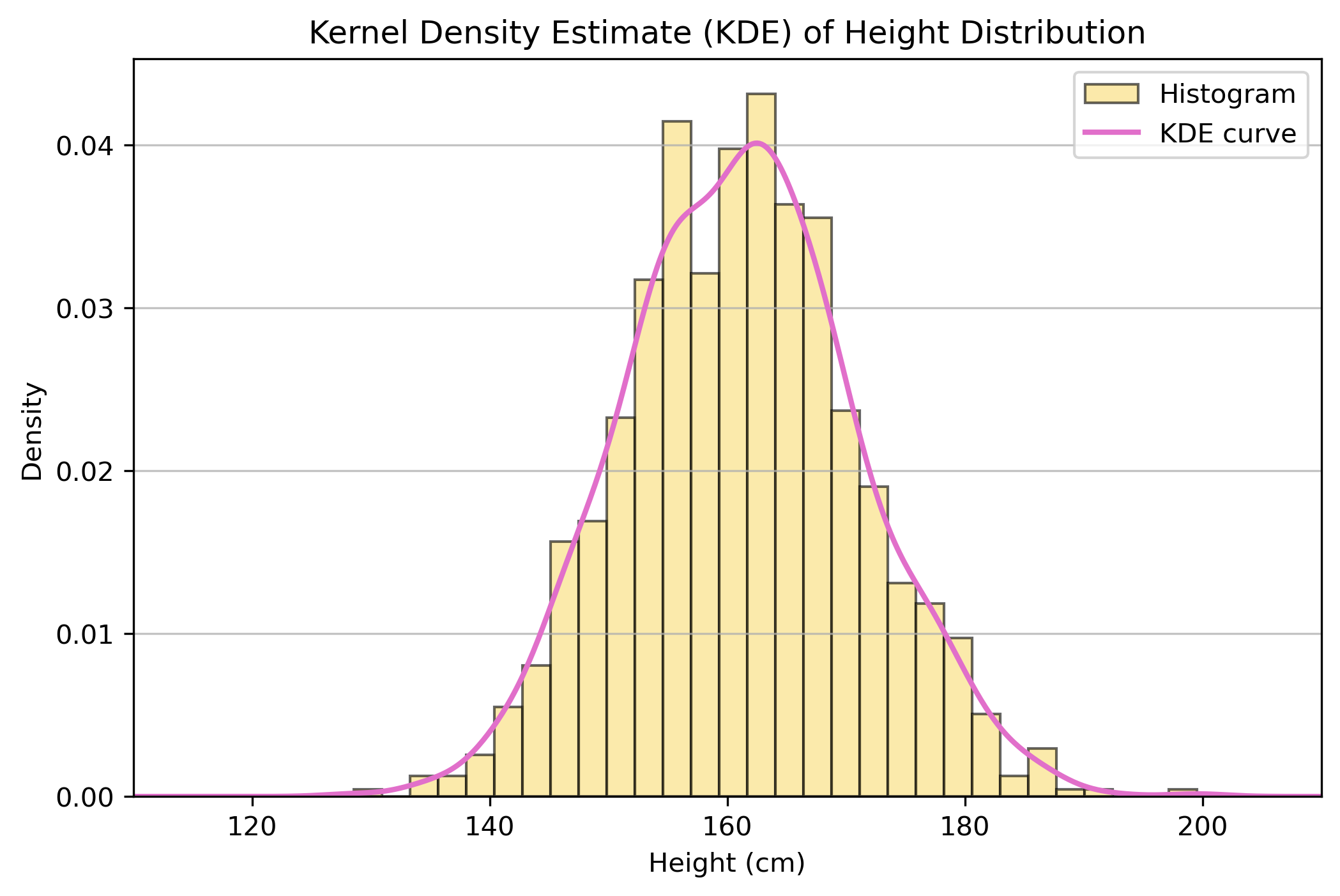
Kernel density estimate (KDE)

• Used to generate a smooth probability density function for a random variable dataset
• Useful for understanding the underlying distribution of a sample
• Think of it as getting a smooth function to describe a histogram of data
• There are no assumptions about the prior distribution

Remember from last week - the probability density function (PDF) describes the likelihood of different outcomes for a continuous random variable

KDE of simulated heights

It’s easy to fit a KDE to data in Python:

import numpy as np
import pandas as pd 
from scipy.stats import gaussian_kde

# Supposing you have some data 
data = pd.read_csv('/path_to_data')

# Kernel Density Estimation
kde = gaussian_kde(data)
x_vals = np.linspace(100, 200, 100)
y_vals = kde(x_vals)

KDE of simulated heights

KDE use case

• fit the KDE to two sample datasets
• compare visually
• carry out a non-parametric test - such as Kolmogorov-Smirnov

How might we use a KDE in practise?

Example: students height

Example - step 1, 2, 3

Define the null and alternative hypothesis

\(H_0\): The mean height of male and female students is the same.

\(H_1\): The mean height of male and female students is different.

Set your significance level

\(\alpha = 0.05\)

Identify the evidence

Group 1 – female students
\(\bar{x}_1 = 170\), \(s_1 = 5\), \(n_1\) = 95

Group 2 – male students
\(\bar{x}_2 = 180\), \(s_2 = 6\), \(n_2\) = 103

Any questions about the steps up to this point?

Example - step 4

Calculate the p-value

• Use Student’s T-test: two sample
  • Don’t care if students are taller or shorter - so use two-tailed test
  • Calculate the t value
  • Calculate the degrees of freedom
  • Get the p value

Example - step 4 - calculate the t value

Substituting values:

\[\begin{align} s_p &= \sqrt{\frac{(95-1)\cdot 5^2 + (103-1)\cdot 6^2}{95+103-2}} \approx 5.55 \end{align}\]

Now compute \(t-value\):

\[\begin{align} t &= \frac{170 - 180}{5.55 \cdot \sqrt{\tfrac{1}{95} + \tfrac{1}{103}}} \approx -12.7 \end{align}\]

Don’t need to know the formulas because in practise we’ll be using Python functions to do the calculations for us.

Using the right python function is something we’ll cover in todays tutorial.

Example - step 4 - calculate the degrees of freedom

For Student’s T-Test we need degrees of freedom:

\[\begin{align} df = n_1 + n_2 - 2 = 95 + 103 - 2 = 196 \end{align}\]

Example - step 4 - calculate the p value

Traditionally this uses look up tables - we’re going to use Python.

from scipy import stats

t_val = -12.7
df = 18

# Two-tailed p-value
p_value_two_tailed = 2 * (1 - stats.t.cdf(abs(t_val), df))

print("Two-tailed p-value:", p_value_two_tailed)

Two-tailed p-value: 2.0151302848603336e-10

Example - step 4 - simplified

We can do all the previous calulations in one step using the `scipy’ library - we’ll practise this in the tutorial.

Example - step 5

Compare p-value with hypothesis level

Now we need to compare the p-value to our siginificance level.

p-value = \(2.0151302848603336e-10 < 0.05\) = alpha

…we reject \(H_0\)!

And conclude that male and female students have significantly different heights.

Questions?

Overview

We’ve covered:

• What makes a good hypothesis
• How to formally state a hypothesis
• Types of statistical tests

Practical

The practical will focus on establishing and evaluating a research hypothesis in python.

Make sure you have questions prepared!