Exploratory Data Analysis 2

Beatrice Taylor - beatrice.taylor@ucl.ac.uk

8th October 2025

Last week

Overview of lecture 1

• Different data types
• Key data metrics
  • the middle and the spread
• Visualising the data
• Data outliers

4 data types: nominal, ordinal, interval, ratio Numerical vs categorical

Key data metrics - the middle: mean, median, mode and the spread: variance and standard deviation

different types of data outliers: caused by measurement error, or irregular pattern or influential outliers

This week

The scientific method

A specific research model - quite formal - been around from the 19th century. Typifies how scientific research is done in the classical sciences like biology. Link to scientific process and how we test and then iterate over ideas and concepts. Something we will talk about more next lecture.

Exploratory data analysis

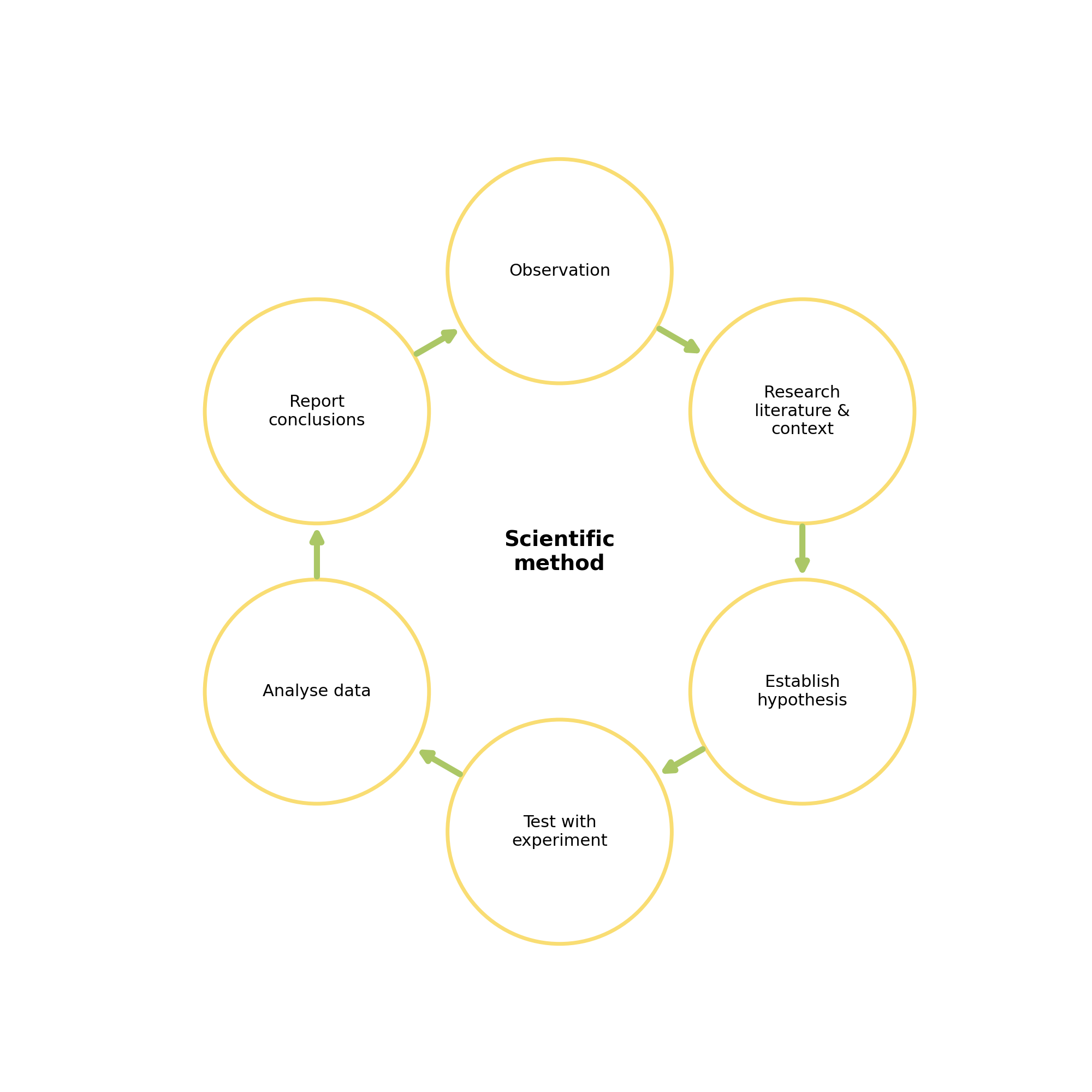
When we’re working with large datasets, exploratory data analysis is the first step in the scientific method.

• How to understand the dataset
• What do the variables represent
• What statistical techniques should be used

More modern approach approach devloped by computer scientist John Turkey in the 1970s - whilst at Princeton. ‘Father of data science’. rather than being driven by more classical statistical analyses (something we’ll look at next week) - the idea was to have a more flexible approach.

Introducing statistical concepts

• Data science is about using ideas from statistics to describe large datasets
• Focus on numerical data
• Using probability distributions to characterise them

In large datasets its not practical to describe every data point - instead interested in the overall pattern. Moreover maybe that general pattern is more interetsing

Learning objectives

By the end of this lecture you should be able to:

1. Describe the characteristic features of common probability distributions.
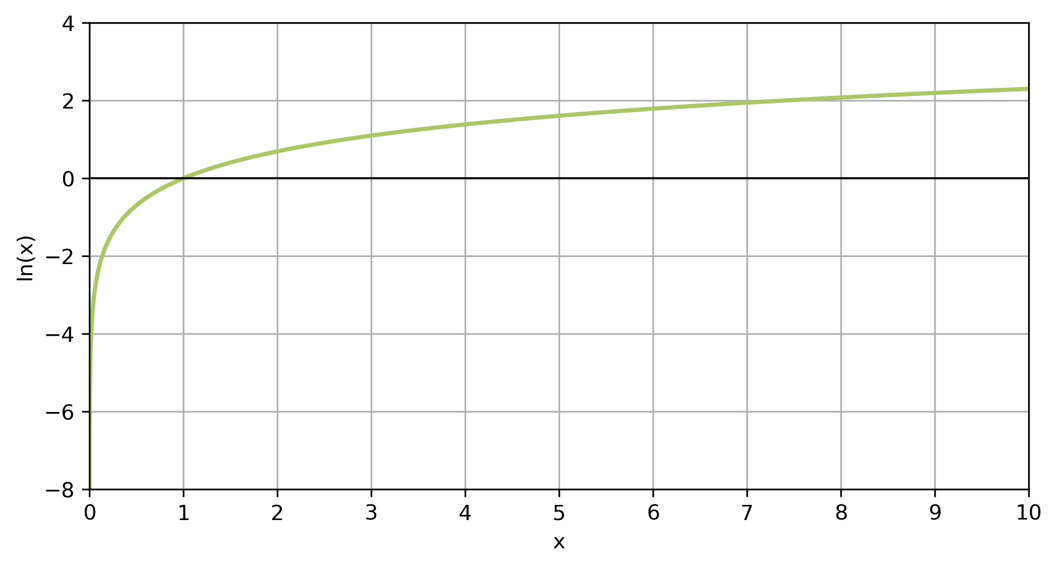
2. Calculate exponentials and logarithms.
3. Evaluate whether a dataset is representative.

Motivation

How do we understand how likely events are to occur?

Question

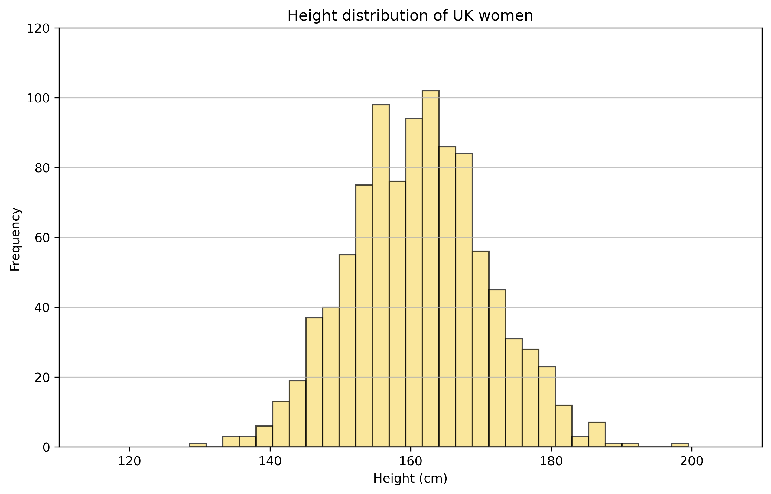
What is the probability of someone at UCL being over 190cm?

How can we try to answer this?

We could try and find someone on campus who is over 190cm.

Better idea is to try and understand the distribution of heights.

This week thinking about the distribution of data. How do we understand the spread of height data, how to we calculate important features of this data, how can we describe this data using mathematical equations?

Next week, thinking about formulating and answering the research question.

Representative data

Before we try to describe the data, it’s important to know where the data came from.

The dream vs reality

Ideally, we would like all the relevant data.

… in reality we normally only have some.

It would be great if I knew the height of everyone at UCL, but unrealistic to collect – however maybe I could collect all students in this lecture theatre.

Approximating

Hence, we sample a subset of the data. We need to choose our sample carefully - we want what happens in the sample to approximate what happens in the whole population.

In practise we might try different sampling approaches such as:

• random sampling
• systematic sampling

I might assign everyone a number and then choose 100 random numbers and measure them. Or I might choose a specific subset, for exampel just everyone in this lecture theatre.

Bias

It’s important to understand if your dataset is unrepresentative or biased.

Bias is the idea that there is an unrepresentative pattern in your data.

Cognitive bias

Systematic patterns in how we think about, and perceive, the world.

Our cognitive biases can impact:

• data collection
• data selection
• data processing
• modelling choices

We all have our own cognitive biases - shaped around our values and our backgrounds. Example of cognitive bias - confirmation bias, whereby I favour information that agrees with my existing beliefs. I’m writing a report on the spatial impact of a new railway line. Suppose I hate the idea of a new railway line, and then I see some data, fact a: 60% of residents living near the railline don’t want it due to noise. fact b: 75% of residents in the UK do want the railway line. i might only include fact a in my report as it confirms my existing beliefs.

Why is this important?

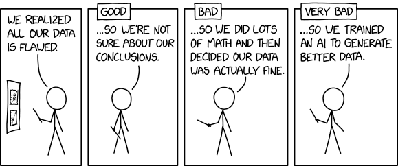
If we’re not careful we can propagate bias to the research, and hence results.

This can lead to incorrect conclusions.

As scientists we should try and present an accurate and fair balance of information. If we’re more aware of our biases it can be easier to try and actively avoid them.

Dataset bias

• Particularly important when thinking about analysing large datasets as there could be non-obvious patterns reflecting biases.
• More important in the era of large AI models

Types of dataset bias include: - Historical bias - Selection bias

Already talked about the idea of cognitive bias. There are lots and lots of different types of biases - going to talk a little about different ways they can bias the dataset.

Dataset bias has become a more prevalent topic of concern on the era of large AI models. These models are really good at learnign patterns which aren’t obvious to the human eye - but the pattern might reflect a bias. For example generative AI models learn that scientists are white men, even though if I asked you you’d tell me anyone can be a scientist.

• Hungry judges

Historical bias

Reflects existing, real world, inequalities

Examples:

• Police profiling
  • Automated tools to detect ‘criminals’.
  • Trained on datasets which reflect current racist practises.

Police profiling models - meant to make easy to spot criminals - but use exisitng crime data - which reflect racist prejudices in society - and the model learns to pick out people of certain ethnic backgrounds.

Tools also used to help the sentnecing of criminals in courts of law - observe the hungry judges effect, where they sentnece differently based on how hungry they are - tend to be harsher just before lunch and more lenient after lunch.

Selection bias

When the sample chosen doesn’t represent the whole population of interest

Examples:

• Self selection Roy Model
  • Underlying characteristics of people who self select into certain groups.
• WEIRD people
  • Commonly sampled in behavioural sciences.
  • Reflects a very small proportion of global population.

Roy model - example from economics - basically there’s not a random selection of people in a specific job - thye have chosen that job based on underlying unobserved characterisitcs. For example suppose I’m interested in wages of workers in different occupations - but they have self-selected into that occupation based on their unique skill set - so it’s a biased representation.

WEIRD = western, educated, industrialised, rich, democratic

Can data ever be truly representative?

Probably not.

Even when we think we have really good data, someone has made the choice to collect this data. Why that data over other data? Does that data reflect their underlying cognitive biases? For example the choice to collect information of peoples opnion about a new trainline might be driven by a political goal of understanding public support for a new government infrastructure project.

Not necessarilly a bad thing, but important to keep in mind. And if the bias is noticeable then it should be acknowledged and reported.

Failing that… .. we can acknowledge our biases!

Image credit: [xkcd](https://xkcd.com/2494/)

Exploring the data - descriptive statistics

What to declare

Descriptive statistics refers to the most basic statistical information about the dataset.

• Sample size (n)
• Mean, median, mode
• Standard deviation
• Range

Example 1

Let’s look at a dataset of students height.

Easy to print the summary statistics in Python, using pandas:

import pandas as pd 

height_df = pd.read_csv("L2_data/heights.csv")
height_df.describe().round(2)

	Height_cm
count	1000.00
mean	161.19
std	9.79
min	128.59
25%	154.52
50%	161.25
75%	167.48
max	199.53

Example 2

Sometimes we need more information.

import pandas as pd 

# read data
df_4datasets = pd.read_csv("L2_data/anscombe_quartet.csv")
# print descriptive statistics
df_4datasets.groupby("dataset").describe()

	x								y
	count	mean	std	min	25%	50%	75%	max	count	mean	std	min	25%	50%	75%	max
dataset
1	11.0	9.0	3.316625	4.0	6.5	9.0	11.5	14.0	11.0	7.500909	2.031568	4.26	6.315	7.58	8.57	10.84
2	11.0	9.0	3.316625	4.0	6.5	9.0	11.5	14.0	11.0	7.500909	2.031657	3.10	6.695	8.14	8.95	9.26
3	11.0	9.0	3.316625	4.0	6.5	9.0	11.5	14.0	11.0	7.500000	2.030424	5.39	6.250	7.11	7.98	12.74
4	11.0	9.0	3.316625	8.0	8.0	8.0	8.0	19.0	11.0	7.500909	2.030579	5.25	6.170	7.04	8.19	12.50

all 4 datasets have very similar descriptive statistics of both the x, and y variables.

Same same but different

These all have mean x = 9, variance x = 11. mean y = 7.5, variance y =4.1.

But we can see from the diagrams that the distribution of the data is very different, some is linear, some is elliptic etc… So we need more advanced ways of describing the data.

Normal distribution

The most fundamental distribution

Also known as Gaussian distribution after Gauss. The shape is known as the bell curve.

• Human height
• Petal size (specifically length of iris petals)
• blood pressure
• birth weight of babies
• measurement errors in science experiments

Key features

You’ve seen it all before

• Data is continuous
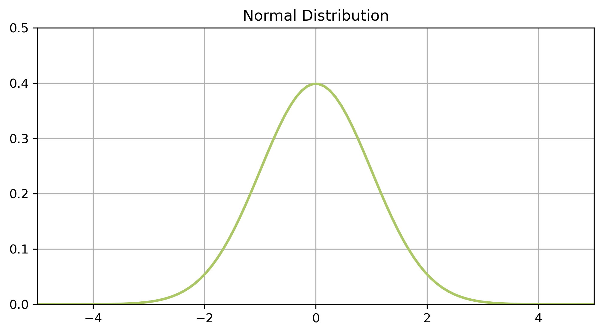
  • it is something you measure not something you count
• Data is equally likely to be larger or smaller than average
  • symmetric
• Characteristic size, all data points are close to the mean
  • single peak
• There is less data further away from the mean
  • smooth tails on both sides

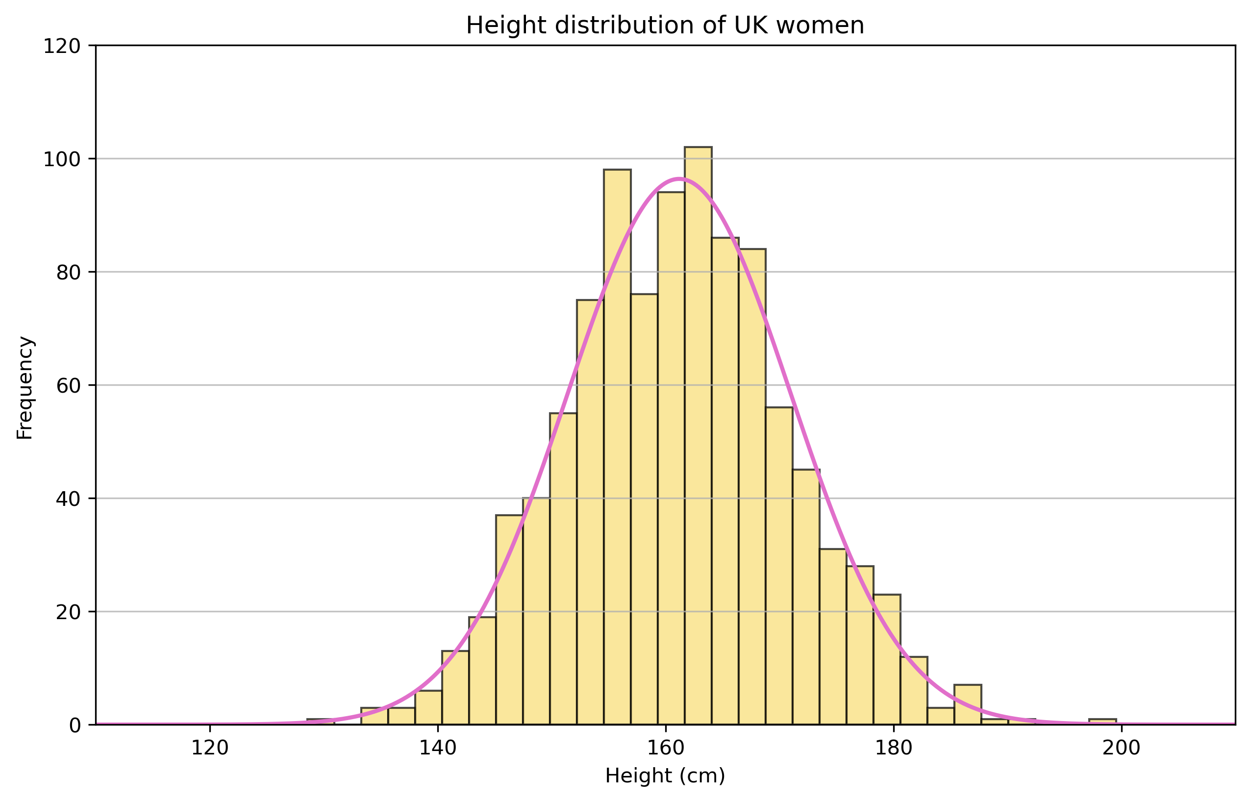
Uniquely described by two variables…

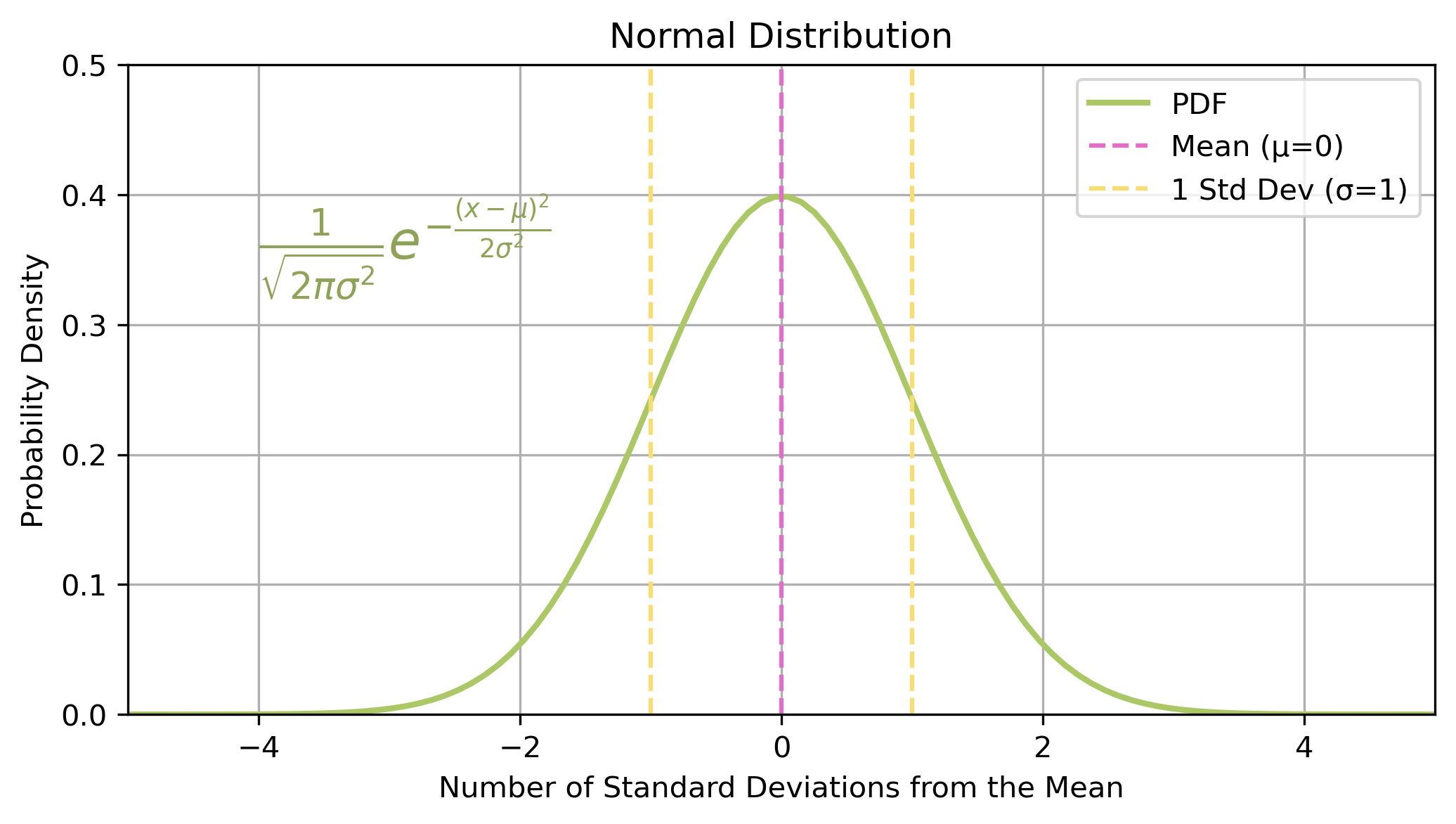
…and a probability distribution function

The probability density function (PDF) describes the likelihood of different outcomes for a continuous random variable

The distribution of the random variable

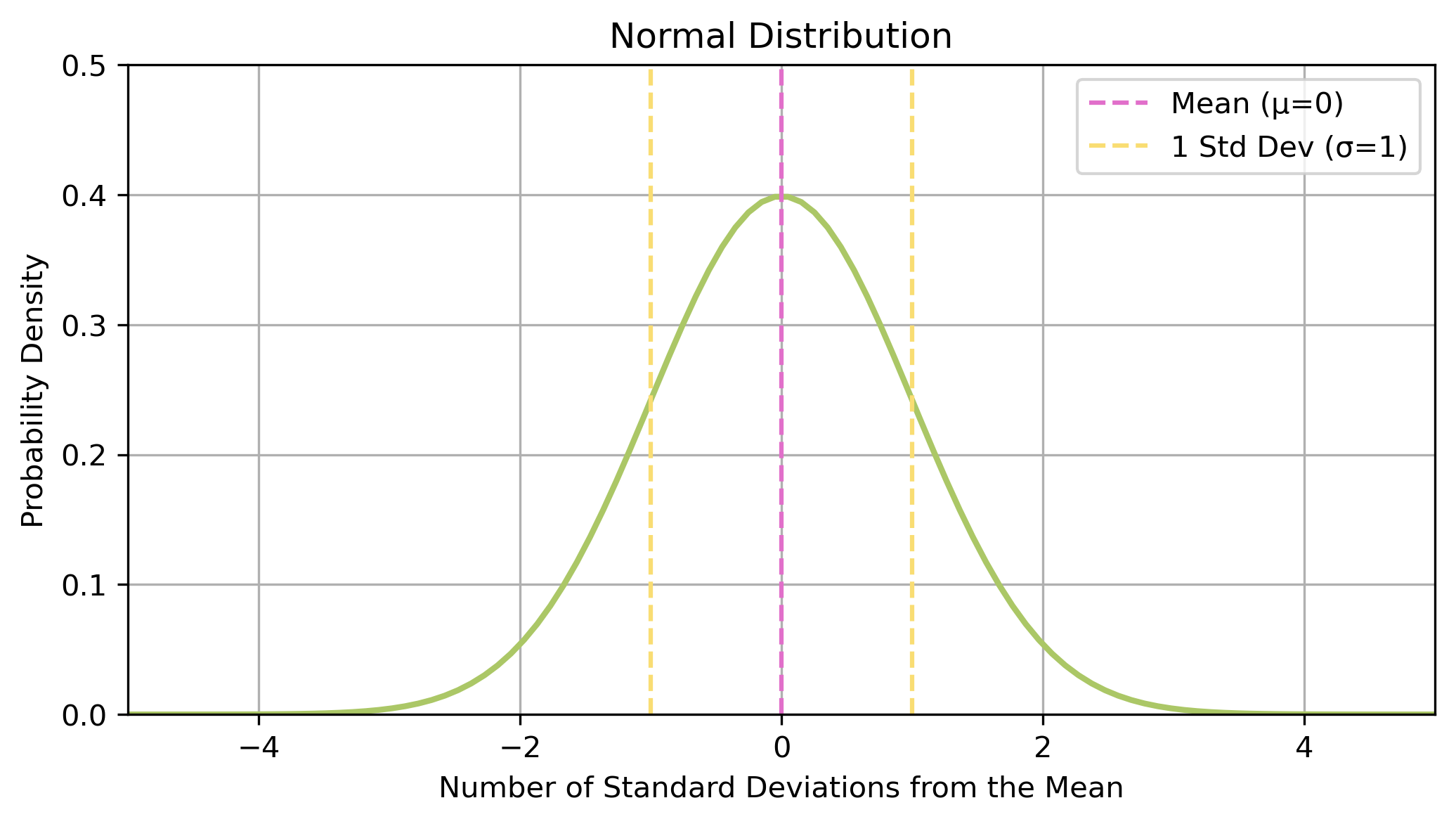
A random variable is a way to map the outcome of a random process to a probability.

In mathematical notation, a random variable \(X\) is approximately normally distributed about a mean of \(\mu\) with a standard deviation of \(\sigma\):

\[\begin{align} X \sim N(\mu,\sigma) \end{align}\]

Sampling distributions

The distribution of the random variable when derived from a random sample of size \(n\)

In the case of the normal distribution the standard deviation becomes:

\[\begin{align} \frac{\sigma}{\sqrt{n}} \end{align}\]

In practise as the sample size increases the sampling distribution becomes more and more centralised.

• i.e. with more data we have more certainty about the distribution.

Typically we think of the distribution as describing the entirety of the relevant popualtion - i.e. every relevant example. Link to sampling - normally only have a subset of the data.

Need to account for the fact that we don’t have all the data. So our statistic will vary a bit according to what sample of the data we’re looking at.

In practise - as the sample size increases the sampling distribution of the normal distribution becomes more and more centralised. I.e. we have more certainty about the distribution.

Calculating probabilities

Can use the PDF to evaluate the probability at a specific point.

\[\begin{align} X \sim N(0,1) \end{align}\]

\[\begin{align} p(x) = \frac{1}{\sqrt{2 \pi \sigma^2}} e^{-\frac{(x-\mu)^2}{2\sigma^2}} \end{align}\]

\[\begin{align} p(x=0.5) = \frac{1}{\sqrt{2 \pi \times 1^2}} e^{-\frac{(0.5-0)^2}{(2\times 1)^2}} \\ = \frac{1}{\sqrt{2 \pi}} e^{-\frac{0.25}{4}} = 0.3747 \end{align}\]

Not everything is normal

Many real world datasets are approximately normally distributed.

But not all

• not continuous
• no characteristic size
• not symmetric

More generally, what is a probability distribution?

Continuous vs. Discrete

Continuous data Measurable data which can take any value within a given range.

example: height

Discrete data Measurable data which can take seperate, countable values.

example: shoe size

Suppose I have someone who is x cm tall, and someone who is y cm tall, I can find someone in between whose x.5cm tall.

But shoe sizes are discrete (not the length of your foot).

Back to the probability function

\[\begin{align} p(x) \end{align}\]

Having a function for the distribution allows us to evaluate the probability of events, and hence evaluate hypotheses.

For discrete distributions we have the probability mass function.

Sampling distributions

As for the normal distribution, in the general case we should be aware of the sampling distribution.

Binomial distribution

Coin toss

• I flip a coin 10 times
• How often can I expect to get at least 7 heads?

Discrete outcomes Describes the frequency of successes in a test with 2 outcomes. Coin flip is the classic example - have exactly two outcomes, either heads or tails.

Probability mass function

\[\begin{align} P(X = k) = \binom{n}{k} p^k (1-p)^{n-k} \end{align}\]

Where \(n\) is the number of trials, and \(p\) is the probability of success for each trial.

The probability mass function (PMF) describes the likelihood of different outcomes for a discrete random variable

Note the combination here.

Plotting the distribution

Example

• I flip a coin 10 times
  • \(n=10\), \(p=0.5\)
• How often can I expect to get at least 7 heads?
  • \(k \geq 7\)

Evaluating the PMF, we get:

\[\begin{align} P(X \geq 7) &= P(X=7) + P(X=8) + P(X=9) + P(X=10) \\ &= 0.1719 \end{align}\]

Poisson distribution

Death by horse kicks

• It’s 1894.
• You’re the statistician Ladislaus Bortkiewicz.
• And you’re wondering,
• How many soldiers in the Prussian army have been killed by horse kicks?

Measuring rare events

• Imagine a situation where certain rare events (like arrival of mail) can occur in an independent fashion.
• The Poisson distribution estimates how many such events are expected within a time interval
• Fixed interval (e.g. one minute)
• Fixed rate of events (\(\lambda\)) (e.g. 4 cars per minute, \(\lambda=4\))
• Poisson distribution gives the probability of \(k\) events.

Typically used to measure rare events like mail arriving or death by horse kicks.

Probability mass function

\[\begin{align} P(X = k) = \frac{\lambda^k e^{- \lambda}}{k!} \end{align}\]

Where \(\lambda\) is the expected number of events in a given interval.

Plotting the distribution

Example

• Between 1883 and 1893 there were an average of 2 deaths from horse kicks a year.
  • \(\lambda=2\)
• What’s the probability of seeing 10 deaths from horse kicks in 1894?

\[\begin{align} P(X = 10) = \frac{2^10 e^{-2}}{10!} \\ = 0.000038 \end{align}\]

Exponentials and Logarithms

Exponentials

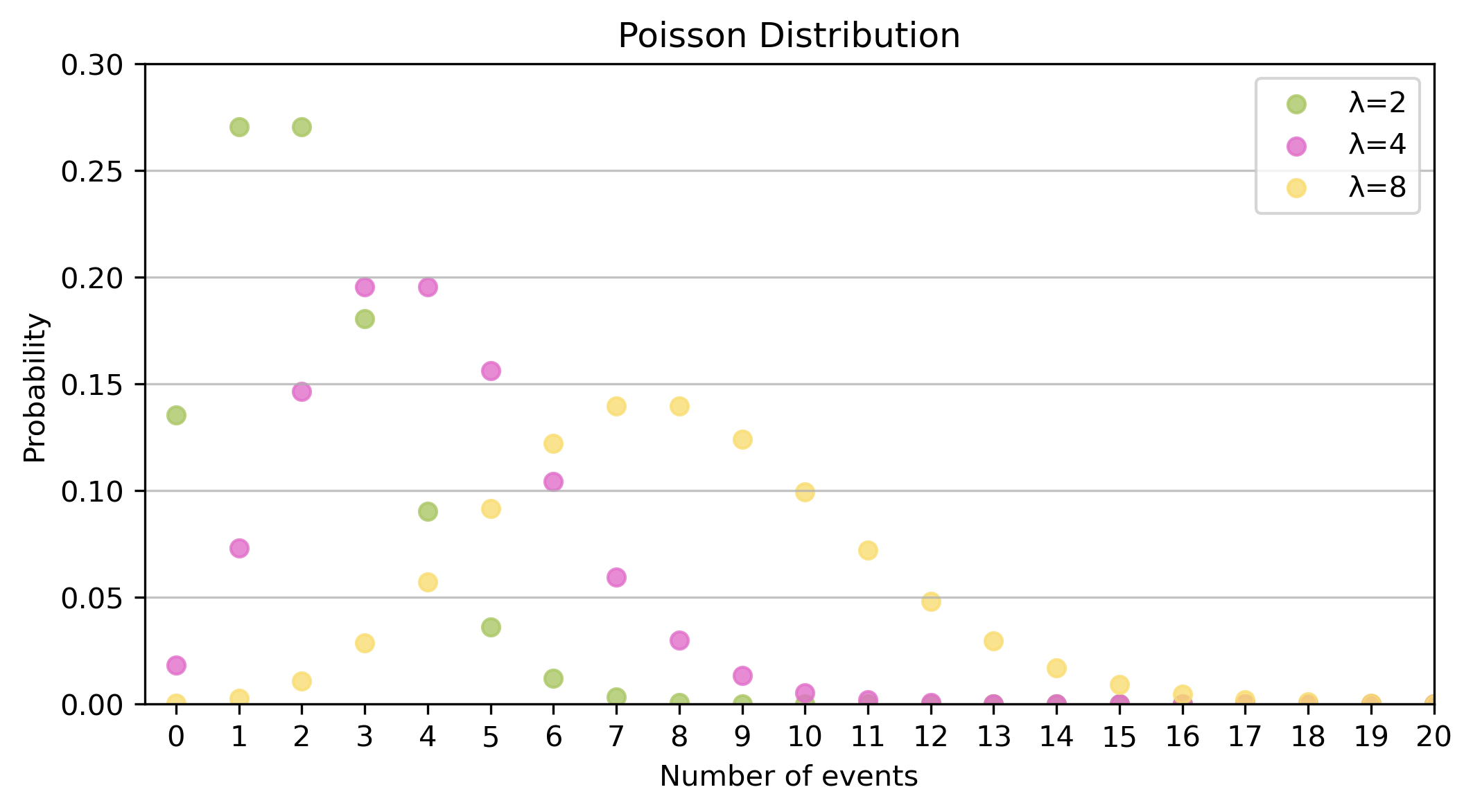
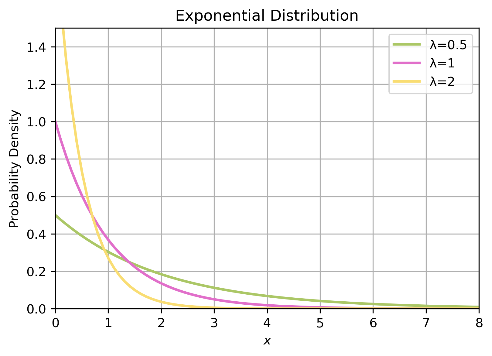
If the Poisson measures the probability of \(x\) events within a time period, then the exponential measures how long we are likely to wait between events.

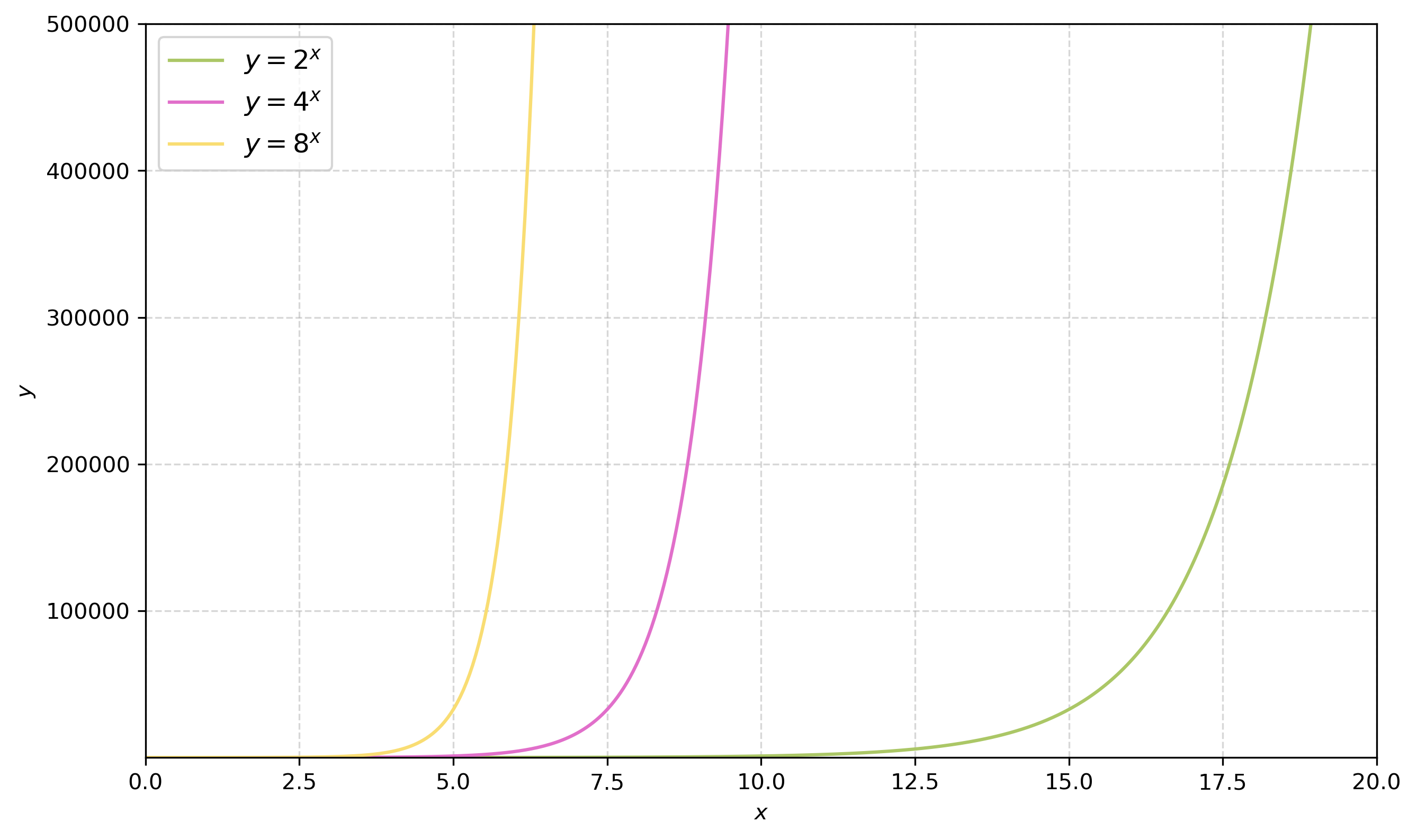
The greatest shortcoming of the human race is our inability to understand the exponential function – Albert Bartlett (physicist)

He’s a bit dramatic

A game of chess…

• A scholar has invented chess
• The emperor is really grateful - and asks what gift the scholar would like in thanks
• The scholar asks for grains of rice
  
• Specifically, rice to fill the chessboard, such that the number of grains double on each square

Image credit: https://simple.wikipedia.org/wiki/Chaturanga

Famous story, of the man who invented chess. Emperor was so grateful, he said what do you want in return The man asked for rice, such that on each square of the chess board, the number of grains of rice doubled. The Emperor thought this was a really small ask for such a great invention. He asked if he didn’t want a better gift. But the man insisted that what he wanted was rice.

Image is of Chatarunga - which is the earliest known form of chess dating to 6th century AD northern India.

…and rice

. . .

10^18

. . .

Which is more than the global production of rice.

A bowl of rice is around 4,000 grains.

What does this look like on a graph?

Generally we have

The exponential function

The (natural) exponential function is:

\[\begin{align} y=e^x \end{align}\]

Note

\(e\) here is eulers number - a mathematical constant.

\[\begin{align} e \approx 2.718... \end{align}\]

Its a mathematical constant similar to pi - it’s just a fixed number which we have a name for. Like pi comes from geometry (circles etc), e comes from the limit of the equation of compound interest.

The exponential distribution

We’ve talked about the exp function - but now want to talk about the exp distribution.

This is a continous probability distribution.

Probability density function

The PDF of the exponential distribution is:

\[\begin{align} f(x, \lambda) = \lambda e^{-\lambda x} \end{align}\]

where \(\lambda\) is the rate parameter. As in the poisson distribution \(\lambda\) is the fixed rates of events for a predetermined time interval.

Note

This is sometimes referred to as the negative exponential distribution - as it’s a negative exponent.

Time between events

Traditionally used to model time between rare events.

• time between volcanic eruptions
• time between customers entering a shop
• time of radioactive decay

Important questions

The exponential allows us to answer questions like:

• What’s the probability that it will be ten years until the next volcanic eruption?
  • \(\lambda=1\)
  • \(p(10) = 1 \times e^{-1 \times 10}\)
• When will the probability of volcanic eruptions be equal to \(p=0.5\)?
  • \(\lambda=1\)
  • \(0.5 = p(x) = 1 \times e^{-1 \times x}\)
  • what is \(x\)?

This is easier said than done – the best way is to invert the equation.

Inverse operations

The mathematical operation that reverses.

Subtract is the inverse of adding.

\[\begin{align} 2 + x=5 \implies 5-2=x \end{align}\]

Divide is the inverse of multiplying.

\[\begin{align} 2 \times x =6 \implies 6 \div 2=x \end{align}\]

Logarithms

Taking the logarithm is the inverse of taking the exponential.

\[\begin{align} 2^3 = 8 \implies \log_2(8) =3 \end{align}\]

More generally:

\[\begin{align} a^x = b \implies \log_a(b) =x \end{align}\]

For the natural logarithm:

\[\begin{align} e^x = b \implies \log_e(b) =ln(b) = x \end{align}\]

Multiply and divide are inverse operations of one another (they reverse the process).

Read the equation as log of 8 base 2 equals 3.

Natural logarithm

Log rules

There are some general rules for how we apply logarithms:

\[\begin{align} log_a(b \times c) &= log_a(b) + log_a(c) \\ log_a(\frac{b}{c}) &= log_a(b)-loc_b(c) \\ log_a(b^c) &= c \times log_a(b) \\ log_a(1)&=0 \\ log_a(a)&=1 \end{align}\]

Transforming data

Some of the most important rules:

\[\begin{align} log_a(a^x) = x \\ ln(e^x) = x \end{align}\]

When we have exponential data we can take the logarithm of it - and hence simplify it.

We will return to the idea of taking the log of data in future weeks - especially in the context of regression analyses.

Overview

We’ve covered:

• Representative data
• Normal distribution
• Binomial distribution
• Poisson distribution
• Exponentials
• Logarithms

Practical

The practical will focus on exploratory data analysis for a variety of different datasets.

Have questions prepared!