This week is focussed on ensuring that you’re able to access the teaching materials and to run Jupyter notebooks locally, as well as describing a dataset in Python.
Learning Outcomes
You have familiarised yourself with how to access the lecture notes and Python notebook of this module.
You have familiarised yourself with running the Python notebooks locally.
You have familiarised yourself with describing a dataset in Python.
Starting the Practical
The process for every week will be the same: download the notebook to your QM folder, switch over to JupyterLab (which will be running in Podman/Docker) and get to work. If you want to save the completed notebook to your Github repo, you can add, commit, and push the notebook in Git after you download it. When you’re done for the day, save your changes to the file (This is very important!), then add, commit, and push your work to save the completed notebook.
Note
Suggestions for a Better Learning Experience:
Set your operating system and software language to English: this will make it easier to follow tutorials, search for solutions online, and understand error messages.
Save all files to a cloud storage service: use platforms like Google Drive, OneDrive, Dropbox, or Git to ensure your work is backed up and can be restored easily when the laptop gets stolen or broken.
Avoid whitespace in file names and column names in datasets
Set up the tools
Please follow the Setup page of CASA0013 to install and configure the computing platform, and this page to get started on using the container & JupyterLab.
Download the Notebook
So for this week, visit the Week 1 of QM page, you’ll see that there is a ‘preview’ link and a a ‘download’ link. If you click the preview link you will be taken to the GitHub page for the notebook where it has been ‘rendered’ as a web page, which is not editable. To make the notebook useable on your computer, you need to download the IPYNB file.
So now:
Click on the Download link.
The file should download automatically, but if you see a page of raw code, select File then Save Page As....
Make sure you know where to find the file (e.g. Downloads or Desktop).
Move the file to your Git repository folder (e.g. ~/Documents/CASA/QM/)
Check to see if your browser has added .txt to the file name:
If no, then you can move to adding the file.
If yes, then you can either fix the name in the Finder/Windows Explore, or you can do this in the Terminal using mv <name_of_practical>.ipynb.txt <name_of_practical>.ipynb (you can even do this in JupyterLab’s terminal if it’s already running).
Running notebooks on JupyterLab
I am assuming that most of you are already running JupyterLab via Podman using the command.
If you are a bit confused with container, JupyterLab, terminal, or Git, please feel free to ask any questions.
Loading data
We are going to describe the population of local authorities in the UK.
We have saved a copy of this dataset to the Github repo, in case that the dataset is removed from the website.
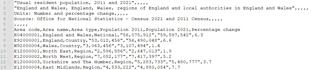
import pandas as pd# Read CSV file, skipping first 5 rows, using row 6 as header, and handling comma as thousands separatordf_pop = pd.read_csv('https://raw.githubusercontent.com/huanfachen/QM/refs/heads/main/sessions/L1_data/UK_census_population.csv', skiprows=5, # Skip first 5 rows. Wnhy? thousands=',', # Interpret commas as thousands separators header=0# After skipping, the first row becomes the header)print(df_pop.head())
   Area code          Area name Area type  Population 2011  Population 2021  \
0  K04000001  England and Wales  National       56075912.0       59597542.0
1  E92000001            England   Country       53012456.0       56490048.0
2  W92000004              Wales   Country        3063456.0        3107494.0
3  E12000001         North East    Region        2596886.0        2647013.0
4  E12000002         North West    Region        7052177.0        7417397.0

   Percentage change
0                6.3
1                6.6
2                1.4
3                1.9
4                5.2
You might wonder why skipping the first 5 rows and setting thousands=‘,’. I knew about this after opening this csv file in a text editor and lots of trial-and-errors.
Then, we check the first few rows of this dataset using df_pop.head().
It is a pain to deal with whitespaces in a column, so good practice is to replace the whitespaces (eg tabs, multiple spaces) within column names with underscore.
df_pop.columns = df_pop.columns.str.replace(r'\s+', '_', regex=True)print(list(df_pop.columns)) # check again
This dataset contains multiple geographies of UK and different geographies are incomparable. We can check the Area_type column:
print(df_pop.Area_type.value_counts())
Area_type
Local Authority    355
Region               9
Country              2
National             1
Name: count, dtype: int64
So there are 355 records of Local Authority, 9 records of Region, 2 of Country, and 1 of ‘National’. For an introduction to these terms, see this article on ONS.
We will focus on the local authorities, so we apply a filter:
There are two pandas functions that give overview of a dataframe. - info(): shows column data types, non‑null counts, and memory usage. - describe(): shows summary statistics for numeric data (count, mean, std, min, quartiles, max) - describe(include='all'): for both numeric data and non‑numeric data (count, unique, top value, frequency).
Now, we focus on describing the local authority population from census 2021. The first question is, what data type is this variable - nominal, ordinal, interval, or ratio?
Note
The data type of a variable is different from how it’s stored in a computer. For example, the Area_type variable can be encoded for convenience as 0 (“national”), 1 (“country”), and 2 (“local authority”). Although these are stored as numbers, Area_type is not truly numeric data — it’s an nominal variable.
Does it make sense to say ‘the population of LA AAA is twice of LA BBB’? Yes. So, this variable is of ratio type.
max and min
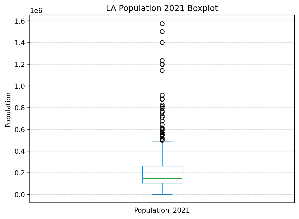
What is the maximum population size in census 2021?
Which LAs have the maximum population size? The code below is a bit complicated.
print("{} have the maximum population of {}".format(", ".join(df_pop_la.loc[df_pop_la['Population_2021'] == df_pop_la['Population_2021'].max(skipna=True), 'Area_name']), df_pop_la['Population_2021'].max(skipna=True)) )
Kent have the maximum population of 1576069.0
What it does:
Finds the max population while ignoring NaNs. It is always safe to use skipna=True, even though there is no NA values.
Selects all rows with that population.
Joins their Area_name values into a comma-separated string.
Two new Python functions here:
format(): Inserts variables into a string by replacing {} placeholders in order with provided arguments.
join(): Combines the elements of an iterable into one string using the given separator before .join().
Which LAs have the minimum population?
print("{} have the minimum population of {}".format(", ".join(df_pop_la.loc[df_pop_la['Population_2021'] == df_pop_la['Population_2021'].min(skipna=True), 'Area_name']), df_pop_la['Population_2021'].min(skipna=True)) )
Isles of Scilly have the minimum population of 2054.0
Standard deviation
The result from df_pop_la.describe() indicates that the standard deviation of Population_2021 is 2.245442e+05.
Another way to calculate this standard deviation and to reformat it is:
std_dev = df_pop_la['Population_2021'].std()# plain notationprint("The standard deviation of Population_2021 is: {}".format(std_dev)) # scientific notationprint("Using scientific notation: {:.3e}".format(std_dev)) # thousands separator notation + 2 decimal placesprint("Using thousands separator notation: {:,.2f}".format(std_dev))
The standard deviation of Population_2021 is: 224544.20636612535
Using scientific notation: 2.245e+05
Using thousands separator notation: 224,544.21
There are several ways to represent numbers, and which one you choose depends on the situation.
Equally important is to ensure the numbers are meaningful, or to use proper significant figures. For example, reporting a population’s standard deviation with 10 decimal places does not make sense.
Null value and outliers?
Are there Null values or outliers in this variable? From results of info(), there are no NA values.
To detect outliers, we will implement the Tukey Fences method using pandas function, as pandas does not provide a built-in function for this method.
print("{} have the largest population percentage change of {}%".format(", ".join(df_pop_la.loc[??['??'] == ??['??'].max(skipna=True), 'Area_name']), df_pop_la['Population_2021'].??(skipna=True)) )
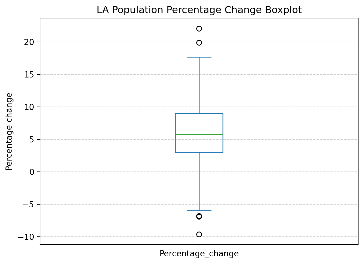
print("{} have the largest population percentage change of {}%".format(", ".join(df_pop_la.loc[df_pop_la['Percentage_change'] == df_pop_la['Percentage_change'].max(skipna=True), 'Area_name']), df_pop_la['Percentage_change'].max(skipna=True)) )
Tower Hamlets have the largest population percentage change of 22.1%
Which LAs experienced the smallest population percentage change? To what extent?
print("{} have the smallest population percentage change of {}%".format(", ".??(df_pop_la.loc[df_pop_la[??] == ??['Percentage_change'].??(skipna=True), 'Area_name']), df_pop_la['Percentage_change'].??(skipna=True)) )
print("{} have the smallest population percentage change of {}%".format(", ".join(df_pop_la.loc[df_pop_la['Percentage_change'] == df_pop_la['Percentage_change'].min(skipna=True), 'Area_name']), df_pop_la['Percentage_change'].min(skipna=True)) )
Kensington and Chelsea have the smallest population percentage change of -9.6%
import matplotlib.pyplot as plt# Create boxplotdf_pop_la[??].plot(kind=??, title='LA Population Percentage Change Boxplot')plt.??('Percentage change')plt.grid(axis='y', linestyle='--', alpha=0.6)plt.show()
import matplotlib.pyplot as plt# Create boxplotdf_pop_la['Percentage_change'].plot(kind='box', title='LA Population Percentage Change Boxplot')plt.ylabel('Percentage change')plt.grid(axis='y', linestyle='--', alpha=0.6)plt.show()
You’re Done!
Congratulations on completing the first QM practical session! If you are still working on it, take you time.
Don’t worry about understanding every detail of the Python code — what matters most is knowing which functions to use for a specific task, like checking minimum and maximum values or generating boxplots, and knowing how to debug when it goes wrong. Remember, practice makes perfect.