Feature Selection for Supervised Machine Learning
Huanfa Chen - huanfa.chen@ucl.ac.uk
09/03/2026
Recap
- Model interpretation is about explaining a trained model, not the data
- Post-hoc explanations can be global (feature importance, PDP, SHAP) or local (LIME, SHAP)
- Permutation importance is better than drop-feature importance and sklearn tree-based feature importance
- SHAP is a unified framework for explaining ML predictions, based on Shapley values from game theory
- These methods are model agnostic
This week
- Focus on feature selection for supervised machine learning models
- Understand the classification of feature selection methods (unsupervised vs supervised)
- Can apply classic feature selection methods for supervised machine learning models
Definition
- Selecting a subset of relevant features for supervised machine learning.
- Features are also called X variables, independent variables, or input variables.
- Why Selecting Features?
- Faster model training
- Lower cost for data collection
- More interpretable model
- Caveat: might compromise model performance if some features are discarded
How many features are needed?
- No golden rule, but some heuristics:
- 10-20 samples per feature (or #features ~ #samples / 10)
- a predefined number of features, usually 10 or 20
- Using elbow method (model performance vs. # features) to decide #features
Two Types of Feature Selection
- Unsupervised FS: based solely on the features, without considering the target variable
- Example: variance-based, covariance-based, PCA, VIF
- Supervised FS: based on the relationship between features and the target variable
- Example: Lasso, mutual information, tree-based feature importance
Note
This classification is different from unsupervised vs supervised machine learning.
Our Selection of Methods
- VIF (for linear models)
- Lasso (for linear models)
- Mutual information (model agnostic)
- Permutation importance (model agnostic)
- RFECV (model agnostic)
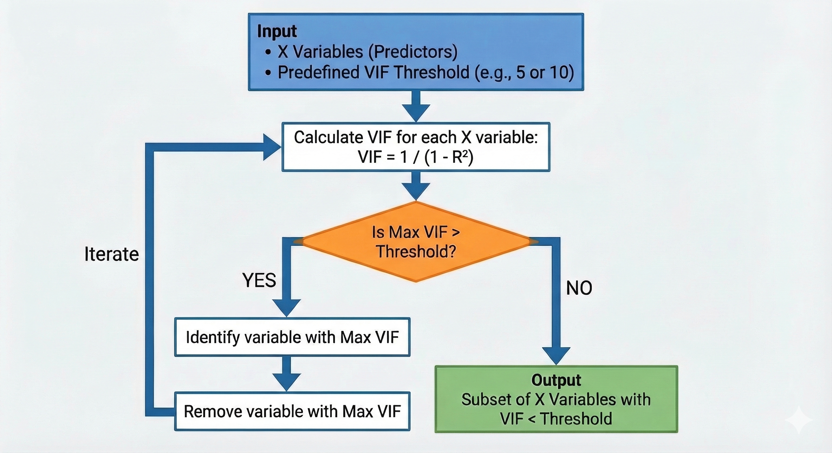
VIF (Variance Inflation Factor)
VIF
- For addressing multicollinearity in linear regression
- Unsupervised feature selection (y is not involved)
- Iterative process. In each step, remove one or zero features
- The VIF of a feature is: \(\text{VIF} = \frac{1}{1 - R^2}\), where \(R^2\) is R2 of a regression of that feature on all the other features.
VIF
VIF Example
Lasso (Least Absolute Shrinkage and Selection Operator)
Lasso definition
- Lasso is a linear regression model with L1 regularisation, which shrinks some coefficients to zero.
- Features with zero coeffcients are effectively removed.
- L1 norm of a vector: \(\|\mathbf{x}\|_1 = \sum_{i=1}^{n} |x_i|\)
- α is hyperparameter that controls regularisation.
- Higher α means more regularisation, which leads to more discarded features.
| OLS | Lasso | |
|---|---|---|
| Formula | \(y = X\beta\) | \(y = X\beta\) |
| To minimise | \(\min_{\beta} \left\{ \frac{1}{2n} \sum_{i=1}^{n} (y_i - \mathbf{x}_i^T \beta)^2 \right\}\) | \(\min_{\beta} \left\{ \frac{1}{2n} \sum_{i=1}^{n} (y_i - \mathbf{x}_i^T \beta)^2 + \alpha \|\beta\|_1 \right\}\) |
Comparing VIF and Lasso
| VIF | Lasso | |
|---|---|---|
| Purpose | Addresses multicollinearity | Feature selection, including address multicollinearity |
| Type | Unsupervised | Supervised |
| When | Before linear regression | Embedded in linear regression |
| Output | Selected features | Features with non-zero coefficients |
| Model Type | Linear regression | Linear regression |
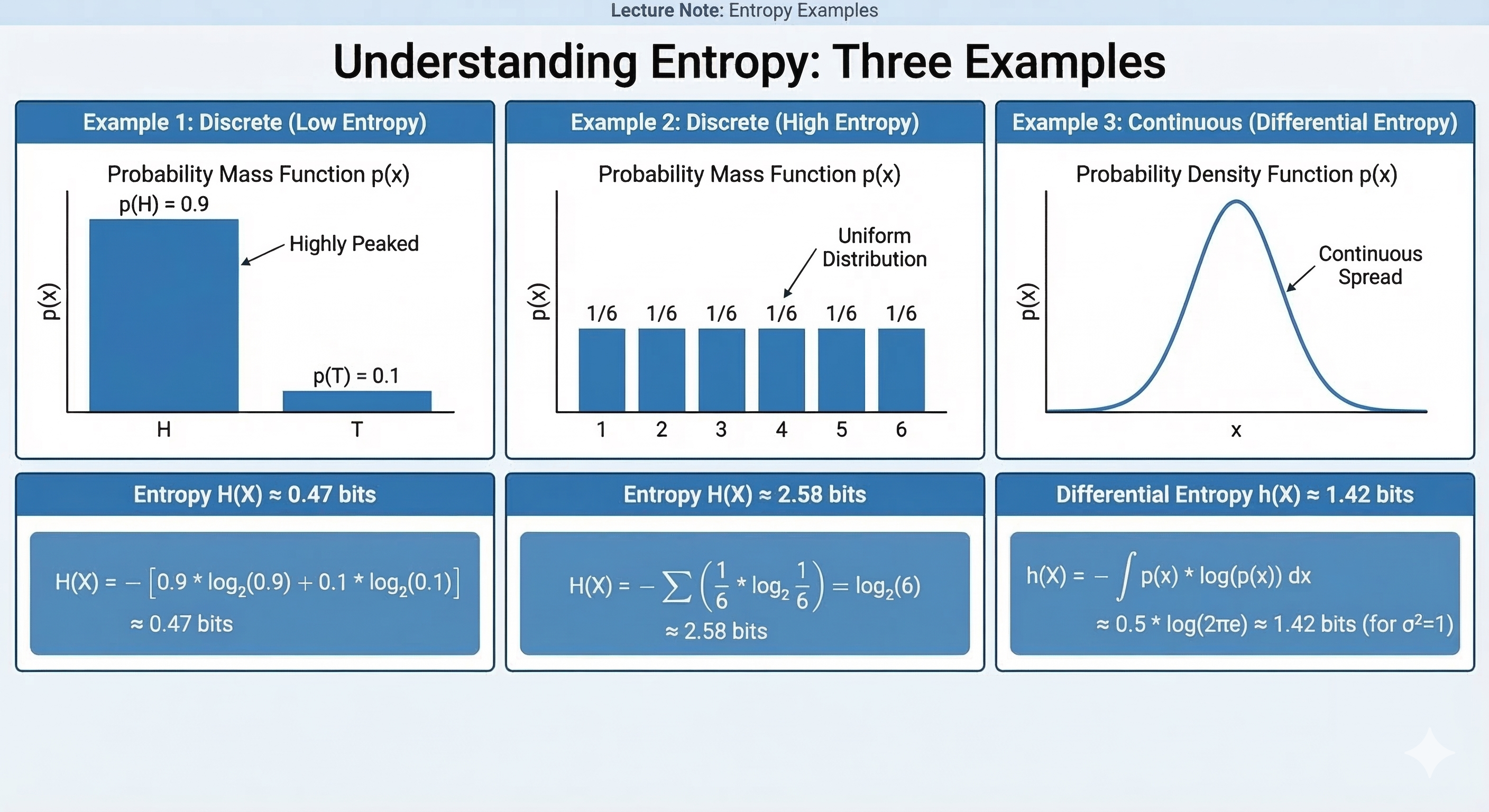
Mutual information
MI definition
- MI measures how much information X and Y share.
- \(I(X; Y) = H(X) - H(X|Y)\), where \(H(X)\) is the entropy (uncertainty) of X, and \(H(X|Y)\) is the conditional entropy of X given Y.
- Entropy of a variable X: \(H(X) = -\sum_{x} P(x) \log P(x)\), where \(P(x)\) is the probability of X taking value x.
MI properties
- MI is similar to Pearson correlation, but more general, as it can capture non-linear relatiionships.
- MI is non-negative. MI=0 means X and Y are independent; higher MI means stronger relationship between X and Y.
- MI is Symmetric: \(I(X; Y) = I(Y; X)\).
- MI is model-independent: similar to Pearson correlation.
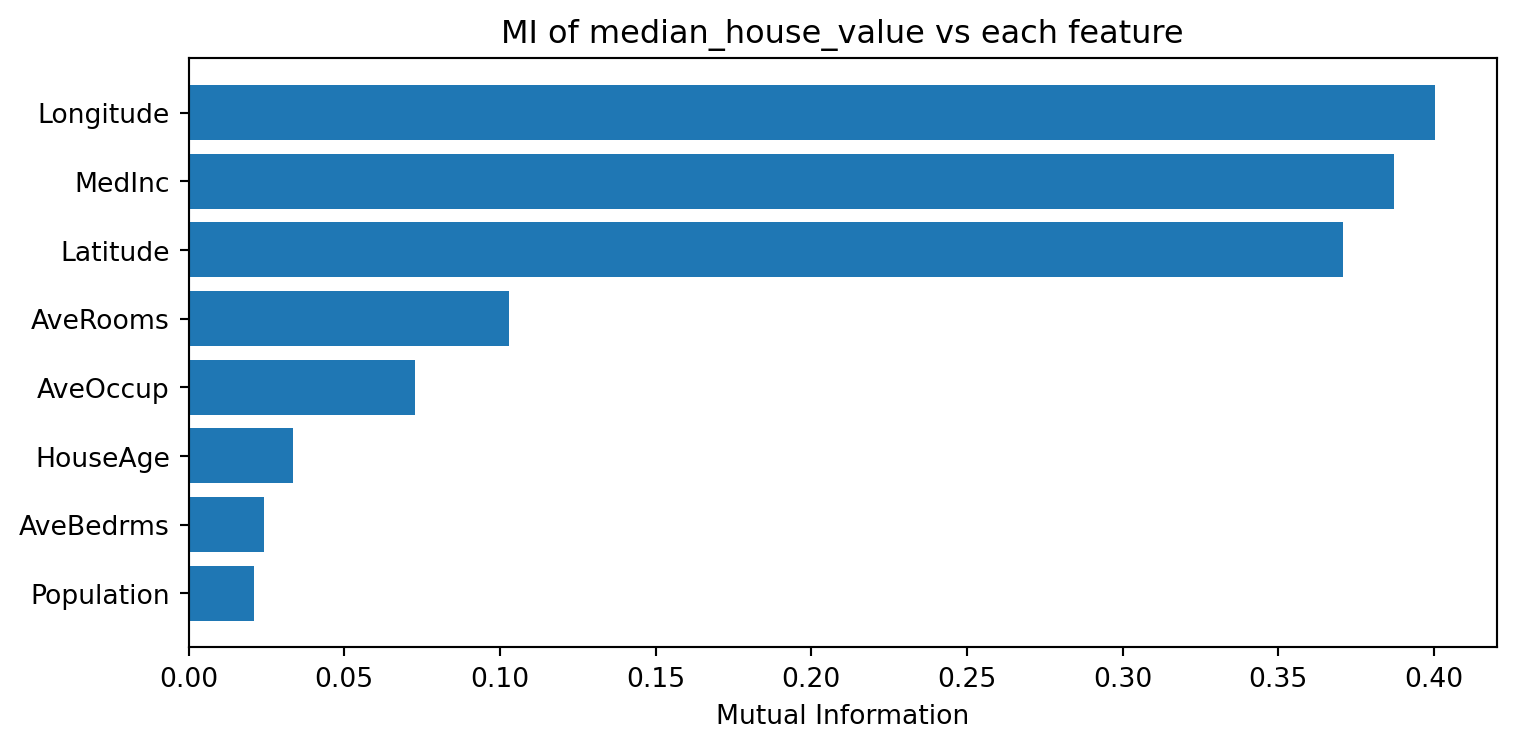
MI example: California Housing
- California housing dataset (from
sklearn): 20,640 houses in California, each described by 8 numeric features (e.g., median income, house age, latitude) - Target variable: median house value (continuous)
MI: median_house_value vs each feature
Using MI for feature selection
- Compute MI between each feature and target variable
- Rank features from highst to lowest MI
- select top k features (e.g. 10) or set a threshold (e.g., MI > 0.1)
- Train the model
Caveats of MI
- Feature redundancy: MI evaluates features one-by-one, so it doesn’t solve multicollinearrity of redundant features. For example, if two features are highly correlated and both are informative (having high MI), they would both be kept.
- Computational cost: MI for continuous variables requires estimating probability distributions, which can be computationally expensive, especially for large datasets or many features.
Permutation importance
Feature importance for feature selection
- Lots of feature importance methods can be used for feature selection
- Permutation importance (model agnostic)
- Tree-based feature importance (only applicable to tree-based models)
- SHAP feature importance (model agnostic)
Permutation Importance Illustration
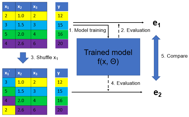
Permutation importance example
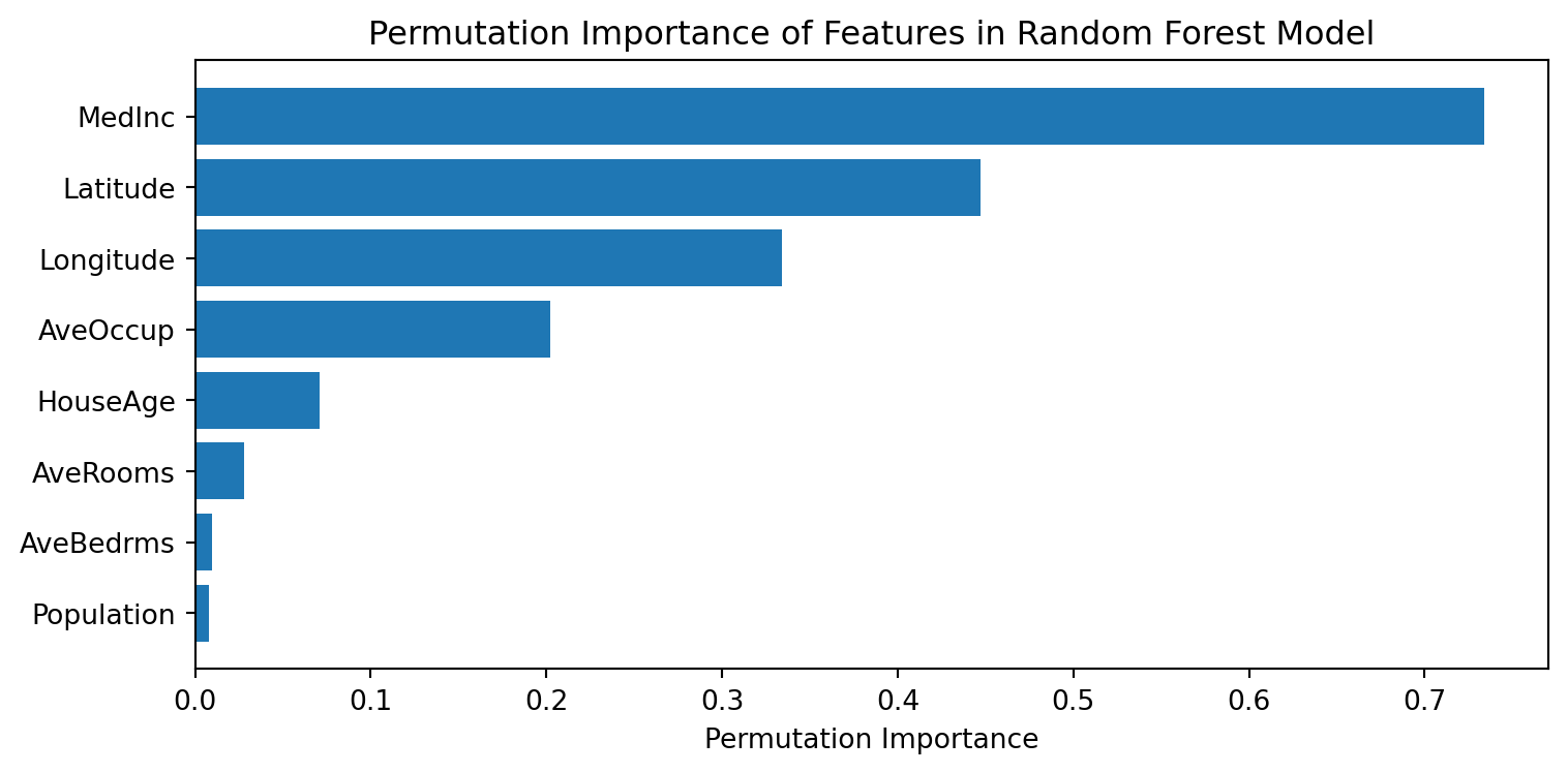
Using PI for feature selection
- Train a model with all features, compute permutation importance, rank features by importance,
- Select top k features (e.g. 10) or set a threshold (e.g. importance > 0.01)
- Train a new model with selected features
RFECV (Recursive Feature Elimination with Cross-Validation)
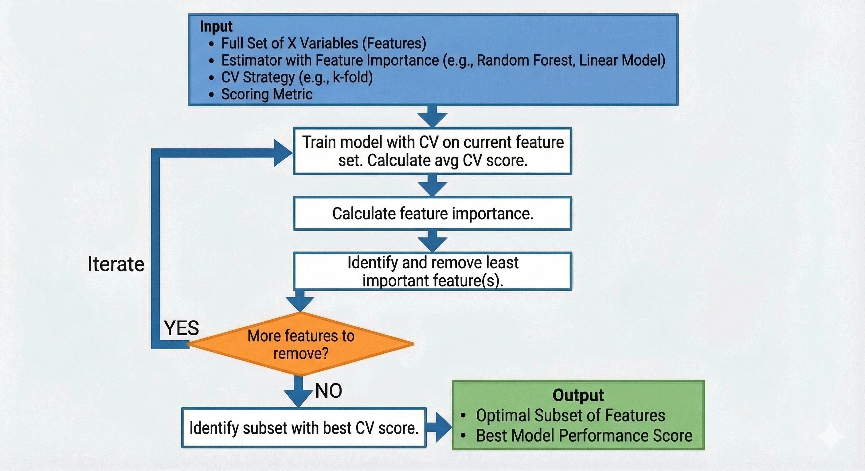
RFECV definition
- A wrapper method for feature selection that recursively eliminates features and uses cross-validation to determine the optimal number of features.
- Should be used with models that have feature importance method, e.g.
coef_orfeature_importances_attribute
RFECV illustration
Advantages & Caveats of RFECV
- Using CV to evaluate model performance with different #features, which is more robust than using training performance
- Can be applied to any model with feature importance
- Caveats: it is computationally intensive as it involves CV and different #features
RFECV example
RFECV example results
- The optimal #features is 8, as n=8 achieves the highest CV R-squared score.
Optimal number of features: 8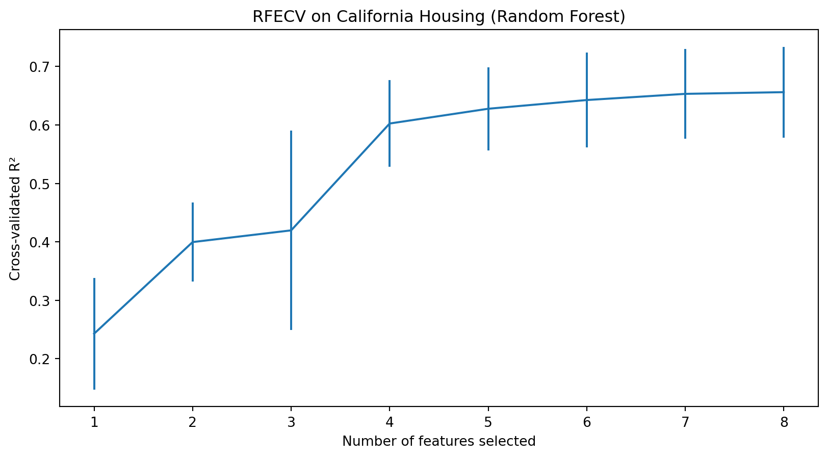
Summary
- We covered five methods for feature selection: VIF, Lasso, mutual information, permutation importance, RFECV.
- For linear regression only: VIF and Lasso
- For supervised machine learning: MI, PI, RFECV
Questions?
![]()
© CASA | ucl.ac.uk/bartlett/casa