Model Interpretation

Huanfa Chen - huanfa.chen@ucl.ac.uk

13/12/2025

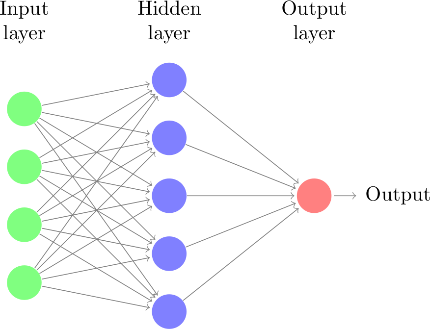
Recap: Neural Networks (or MLP)

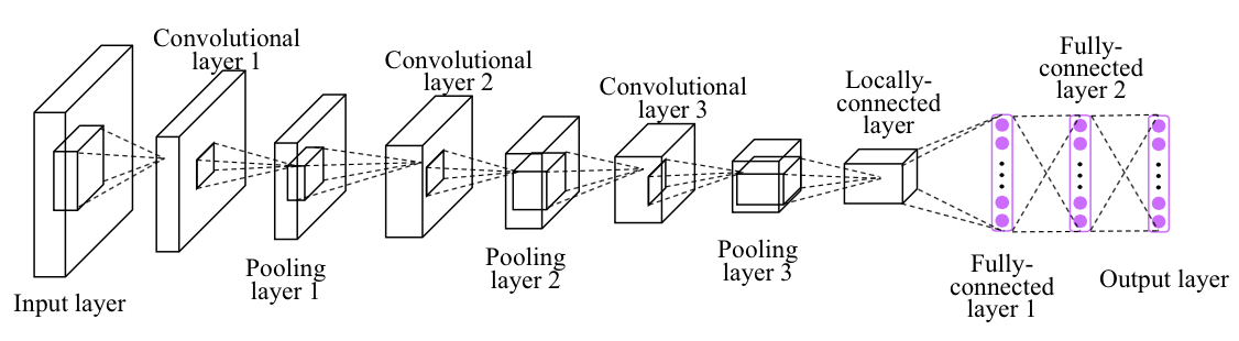
Recap: Convolutional Neural Networks (CNN)

• Local filter
• Translation invariance

source: Arden Dertat

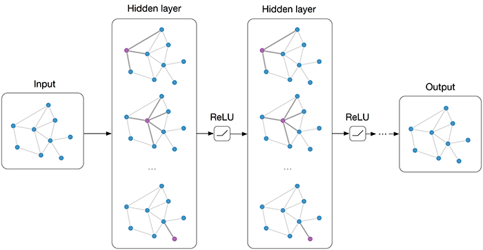
Recap: Graph Neural Networks (GNN)

From this week …

• No new algorithms
• More on how to apply and interpret models
• W07: Model interpretation techniques
• W08: Feature selection methods
• W09: Testing ML codes
• W10: Handling imbalanced data

Model Interpretation (Post-hoc Explanability)

• It involves taking a pre-trained model and using a separate method to explain its decisions
• It belongs to a broader field of Interpretable Machine Learning and Explainable AI (XAI)
• It differs from interpretable models (e.g., linear regression, decision trees), which are designed to be inherently interpretable

What Post-hoc Explanability isn’t …

• This is NOT inference or estimating variable relationships
• This is NOT causality
• Still useful for feature selection and understanding black-box model behaviours

Explaining the Model != Explaining the Data

• Model inspection only tells you about the model
• The model might not accurately reflect the data
• Don’t explain a model with low accuracy

Two types of Post-hoc Explanations

Explain model globally

• How does the model depend on each feature?
• Often in some form of marginals (e.g., feature importance)
• Note that there many types of “feature importance” and they can give very different results!
• Always ask one question: “what is the definition of feature importance?”

Explain model locally

• Why did it classify this data point this way?
• Explanation will be different for each point
• “What is the minimum change to classify it differently?”

Methods

Global:

• Coefficients (❌)
• Sklearn feature importance (❌)
• Drop-feature importance (❌)
• Permutation importance (✔️)
• Partial dependence plots (✔️)

Local:

• LIME (✔️)
• SHAP values (✔️)

Permutation Importance

Idea: measure marginal influence of a feature by permuting it and measuring the drop in accuracy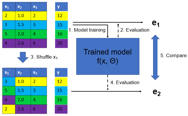

Permutation Importance

\[I_i^\text{perm} = \text{Acc}(f, X, y) - \mathbb{E}_{x_i}\left[\text{Acc}(f(x_i, X_{-i}), y)\right]\]

def permutation_importance(est, X, y, n_repeat=100):
  baseline_score = estimator.score(X, y)
  for f_idx in range(X.shape[1]):
      for repeat in range(n_repeat):
          X_new = X.copy()
          X_new[:, f_idx] = np.random.shuffle(X[:, f_idx])
          feature_score = estimator.score(X_new, y)
          scores[f_idx, repeat] = baseline_score - feature_score

• Stay with the same trained model
• Model agnostic (works for any ML model)
• Can deal with correlated features better
• Can maintain the distribution of a feature
• Can run slow (need to re-evaluate models many times: n_features * n_repeats model evaluations)

Alternatives of permutation importance

• Drop-feature importance (not recommended)
• Idea: to measure importance of x1 for y=f(x1, x2, x3), it drops x1 and refits y=g(x2, x3), and then compare accuracy of f() and g()
• It refits a new model for each feature removal
• Doesn’t really explain model (refits for each feature)
• Can’t deal with correlated features well

Alternatives of permutation importance

• sklearn tree-based feature importance
• Only applicable to tree-based models in sklearn
• For a tree: FI = total reduction of the criterion (e.g., Gini, MSE) brought by that feature
• For a forest: average FI over all trees

Problems with sklearn tree-based feature importance

• Biased towards high-cardinality features (cardinality = number of unique values)
• Can be misleading when features are correlated
• Not recommended

from sklearn.ensemble import RandomForestRegressor
model = RandomForestRegressor()
model.fit(X_train, y_train)
importances = model.feature_importances_ # sklearn tree-based feature importance
PI = permutation_importance(model, X_train, y_train, n_repeats=10,
                                random_state=0) # permutation importance

Partial Dependence Plots

• Marginal dependence of prediction on one (or two) features across differnt values

\[f_i^{\text{pdp}}(x_i) = \mathbb{E}_{X_{-i}}\left[f(x_i, x_{-i})\right]\]

• Idea: Get marginal predictions given feature
• How? “Integrate out” other features using validation data

PDP

from sklearn.inspection import plot_partial_dependence
boston = load_boston()
X_train, X_test, y_train, y_test = train_test_split(boston.data, boston.target,random_state=0)

gbrt = GradientBoostingRegressor().fit(X_train, y_train)

fig, axs = plot_partial_dependence(gbrt, X_train, np.argsort(gbrt.feature_importances_)[-6:], feature_names=boston.feature_names)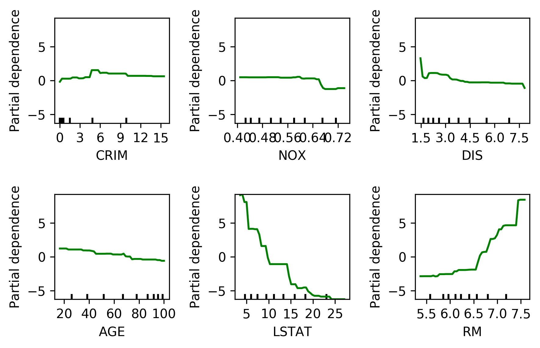

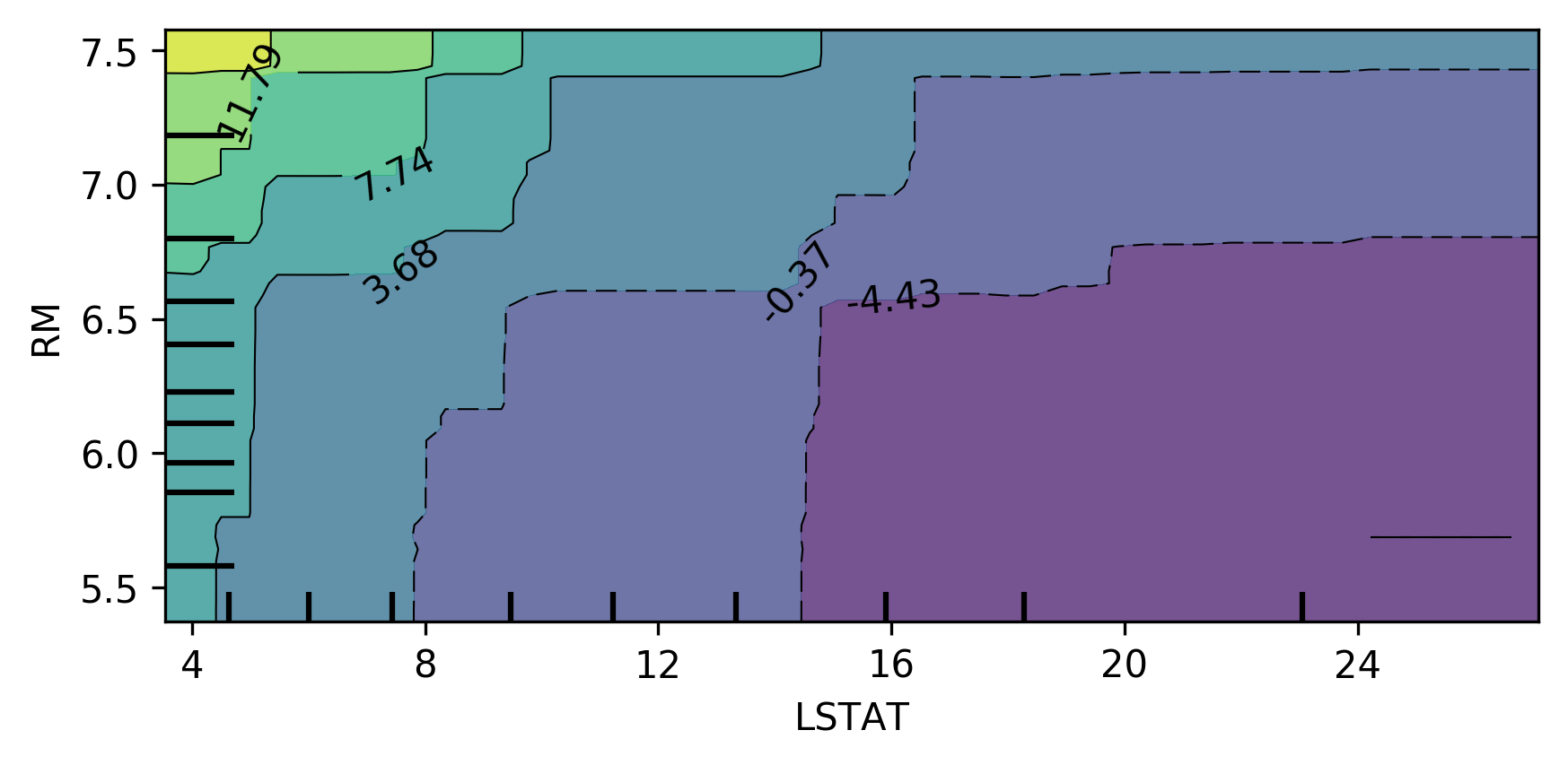
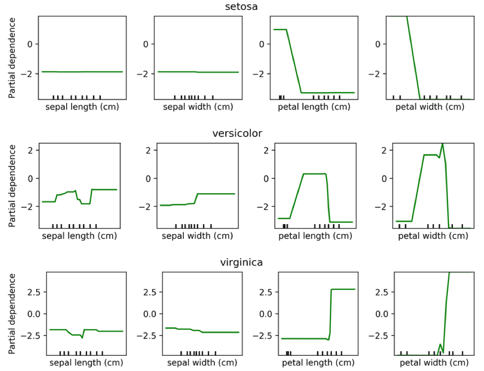
Bivariate Partial Dependence Plots

plot_partial_dependence(
    gbrt, X_train, [np.argsort(gbrt.feature_importances_)[-2:]],
    feature_names=boston.feature_names, n_jobs=3, grid_resolution=50)

Partial Dependence for Classification

from sklearn.inspection import plot_partial_dependence
for i in range(3):
    fig, axs = plot_partial_dependence(gbrt, X_train, range(4), n_cols=4,
                                       feature_names=iris.feature_names, 
                                       grid_resolution=50, label=i)

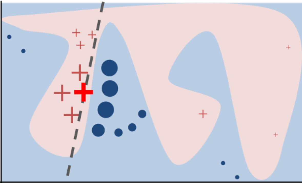
LIME

• Build sparse linear local model around each data point
• Explain prediction for each point locally
• Paper: “Why Should I Trust You?” Explaining the Predictions of Any Classifier
• Implementation: ELI5, https://github.com/marcotcr/lime

SHAP

• Build around idea of Shapley values (from game theory, proposed by Lloyd Shapley in 1953)
• Shapley values: a fair way to distribute “payout” among N players in a game, based on their marginal contributions across all possible coalitions

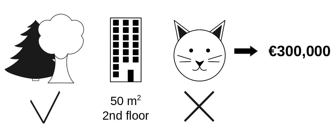
Shapley value

• A fair way to distribute “payout” among N players in a game
• Example in housing price: how much does each factor contribute to the house price?
• What we want to see: park-nearby contributed €30,000; area-50 contributed €10,000; floor-2nd contributed €0; cat-ban contributed -€50,000. But HOW?

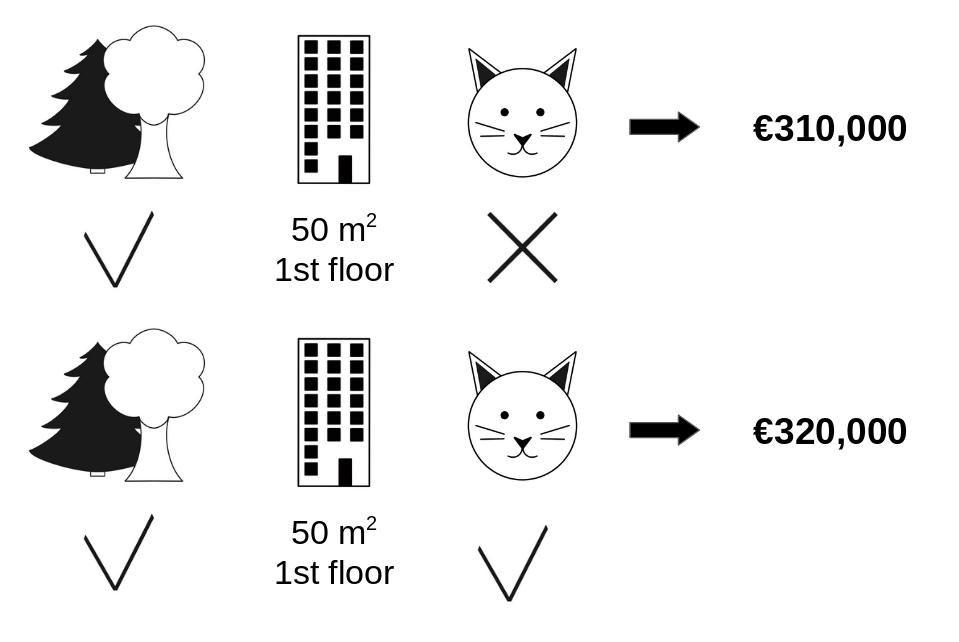
Shapley value (cont.)

• Checking all possible coalition …

Shapley value (cont.)

• To compute payout for cat-ban, we need to check all combinations (with & without cat-ban), and take the difference in predicted price. This payout is (weighted) average of these differences across all combinations.
• If a feature is not in the coalition, we replace it with some baseline (e.g. mean).
  • park-nearby, area-50, floor-2nd
  • park-nearby, area-50
  • park-nearby, floor-2nd
  • area-50, floor-2nd
  • park-nearby
  • area-50
  • floor-2nd
  • {} (empty coalition)

Shapley value (Let’s try again)

• Assume 4 players, to compute Shapley value for player 1:
  • Consider all subsets of players not including player 1: {}, {2}, {3}, {4}, {2,3}, {2,4}, {3,4}
  • For each subset S, compute marginal contribution of player 1: \(v(S ∪ {1}) - v(S)\)
  • Weight each marginal contribution by the number of ways to arrange players in S and N \ S \ {1}
  • Sum weighted contributions to get φ₁(v)

Shapley value

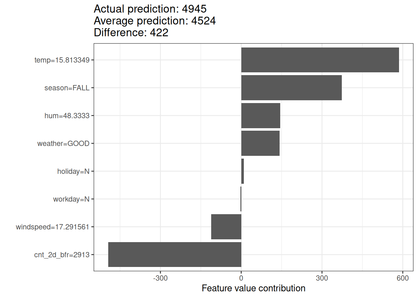
• Example of Shapley value for bike rental prediction
• The sum of Shapley values yields the difference of actual and average prediction (422).
• The temperature & humidity had the largest positive contributions.

Shapley value (game theory)

• Shapley value is the only attribution method that satisfies following properties
• Efficiency: sum of attributions = difference between actual output and average output
• Symmetry: if two features contribute equally, they get same attribution
• Dummy: if a feature does not affect the output, its attribution is zero
• Additivity: for two models, attributions add up. (Think about a random forest with many trees, the Shapley values of the forest is the avereage of SHAP values of each tree)

From Shapely values to SHAP

• SHAP (SHapley Additive exPlanations) is a unified framework for explaining ML predictions, based on Shapley values
• Shapely values were proposed in 1953
• In 2017, Lundberg and Lee proposed SHAP for explaining ML models.
  • assume the explanation as a linear model of binary variables indicating presence/absence of features
  • allows local / per sample explanations, and global explanations (by averaging)
  • introduced effecient estimation of KernelSHAP and TreeSHAP

SHAP

SHAP assumes the prediction of a data point is the sum of effects of each feature. It defines:

\[g(z') = \phi_0 + \sum_{i=1}^{M} \phi_i z'_i\]

• \(\phi_0\): The base value (the average prediction of the model across the dataset).
• \(\phi_i\): The SHAP value (the contribution of feature \(i\)).
• \(z'_i \in \{0, 1\}^M\): A binary vector representing whether a feature is present or absent.
• \(M\): The number of input features.

Computing SHAP

• The original Shapley values are computationally expensive (exponential in number of features)
• SHAP introduced efficient estimation methods:
• KernelSHAP: model-agnostic, uses sampling to estimate SHAP values (model agnostic)
• Permutation SHAP: approximate method using permutations, similar to permutation importance
• TreeSHAP: efficient exact computation for tree-based models

SHAP example

• Y variable: median house value for California districts (in $100,000)

Feature	Description
MedInc	Median income in block group
HouseAge	Median house age in block group
AveRooms	Average number of rooms per household
AveBedrms	Average number of bedrooms per household
Population	Block group population
AveOccup	Average number of household members
Latitude	Block group latitude
Longitude	Block group longitude

• Spatial unit: A block group typically has a population of 600 to 3,000 people; similar to output area in UK
• Source: https://www.dcc.fc.up.pt/~ltorgo/Regression/cal_housing.html

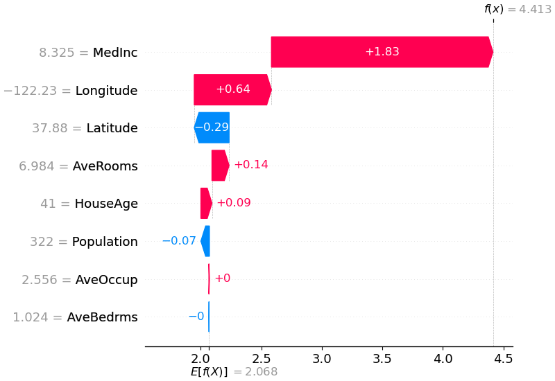
SHAP waterfall plot

import xgboost
import shap

X, y = shap.datasets.california() # 20640 instances, 8 features
model = xgboost.XGBRegressor().fit(X, y)

explainer = shap.Explainer(model)
shap_values = explainer(X)
shap.plots.waterfall(shap_values[0])

SHAP force plots

shap.plots.force(shap_values[0])

SHAP force plots for multiple samples

shap.plots.force(shap_values[:500])

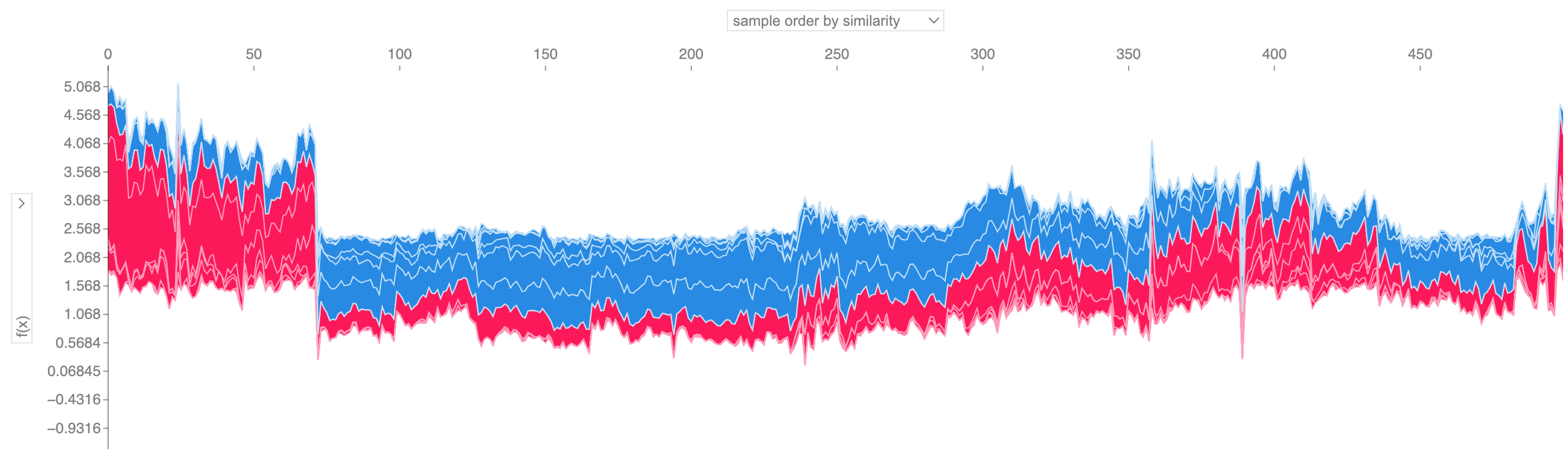
• Use with caution!

SHAP Summary Plot

shap.plots.beeswarm(shap_values)

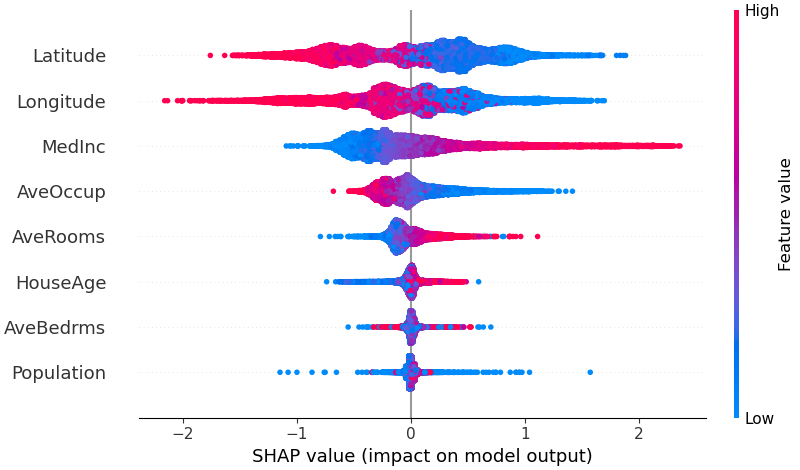
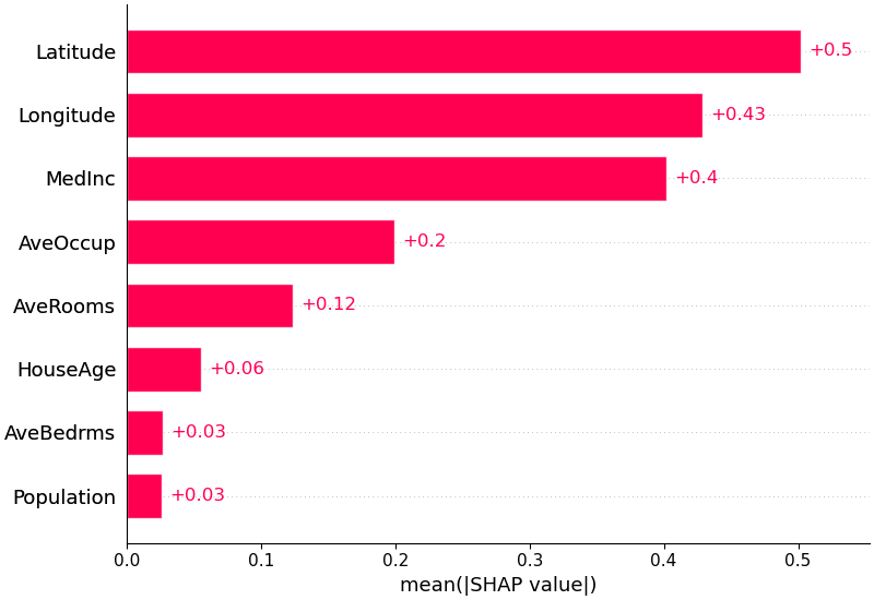
SHAP Feature Importance

• Defined as the mean absolute values of SHAP across all samples

shap.plots.bar(shap_values)

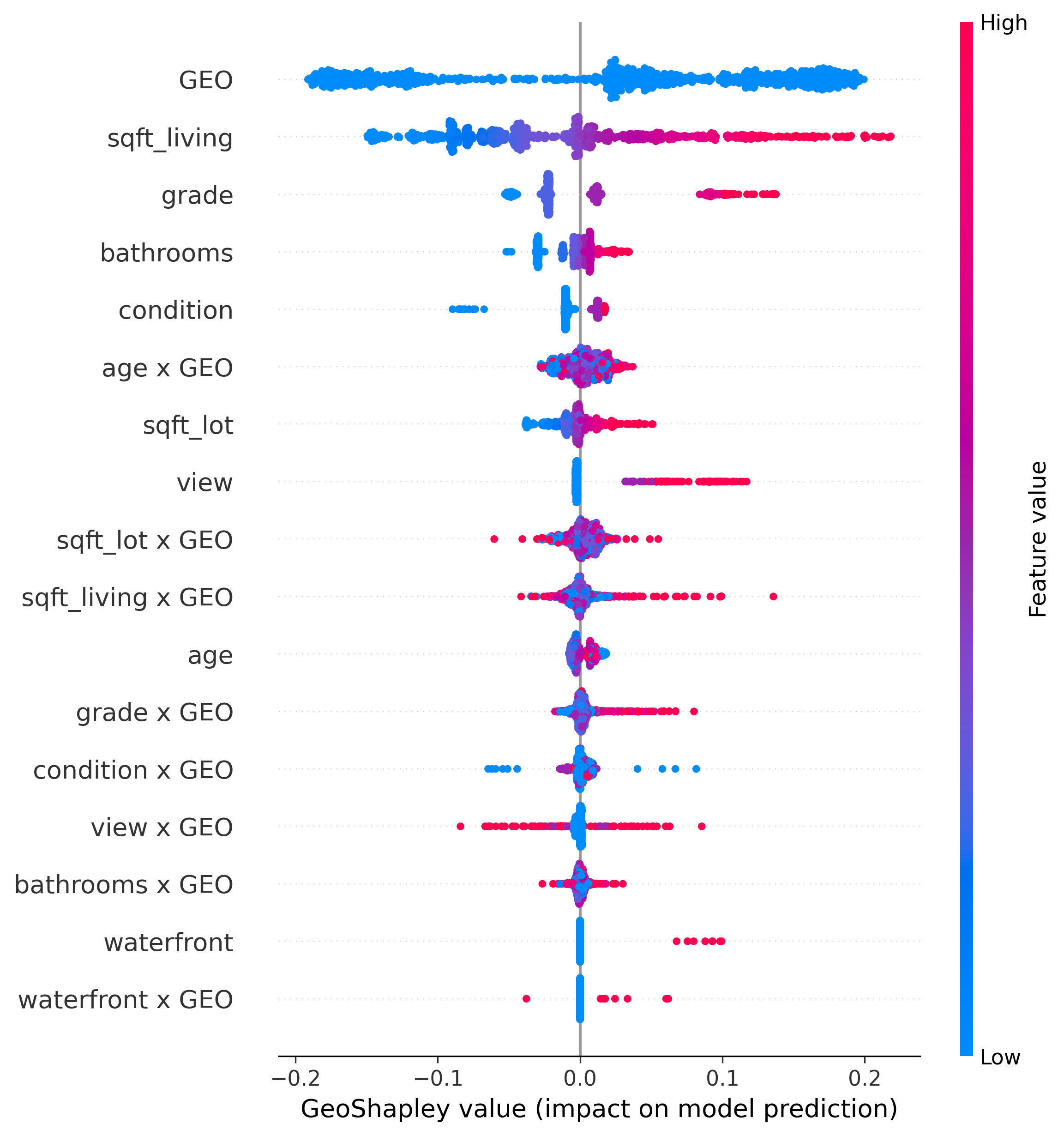
GeoShapley

• Explains any model that takes tabular data + spatial features (e.g., coordinates)
• Source: https://github.com/Ziqi-Li/geoshapley

Key Takeaways

• Model interpretation is about explaining a trained model, not the data
• Post-hoc explanations can be global (feature importance, PDP, SHAP) or local (LIME, SHAP)
• Permutation importance is better than drop-feature importance and sklearn tree-based feature importance
• SHAP is a unified framework for explaining ML predictions, based on Shapley values from game theory
• SHAP is different from Shapley values!
• These methods are model agnostic

Questions?