Graph Neural Networks

Extending neural networks to graph-structured data

Huanfa Chen - huanfa.chen@ucl.ac.uk

13/12/2025

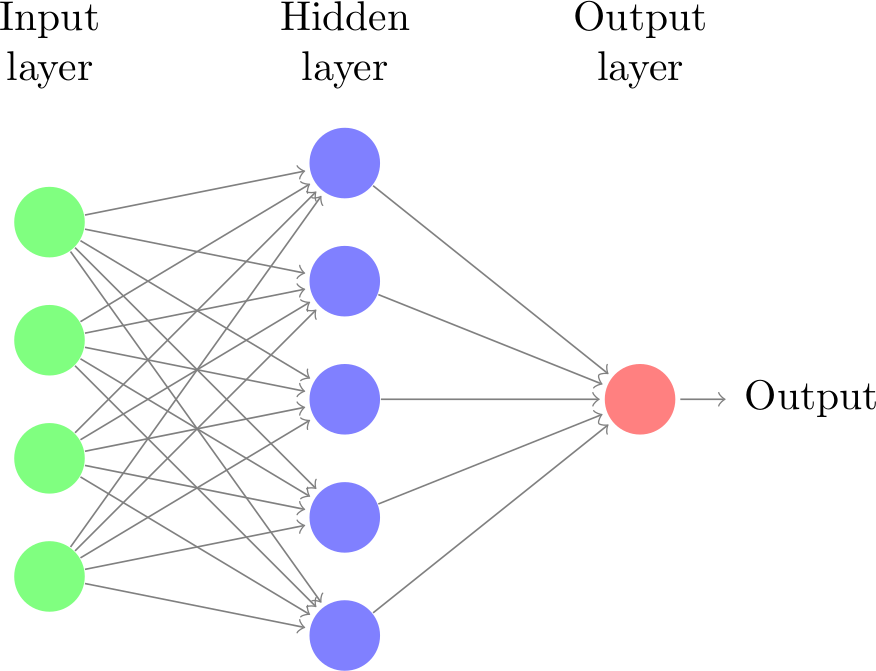
Recap: Neural Networks (or MLP)

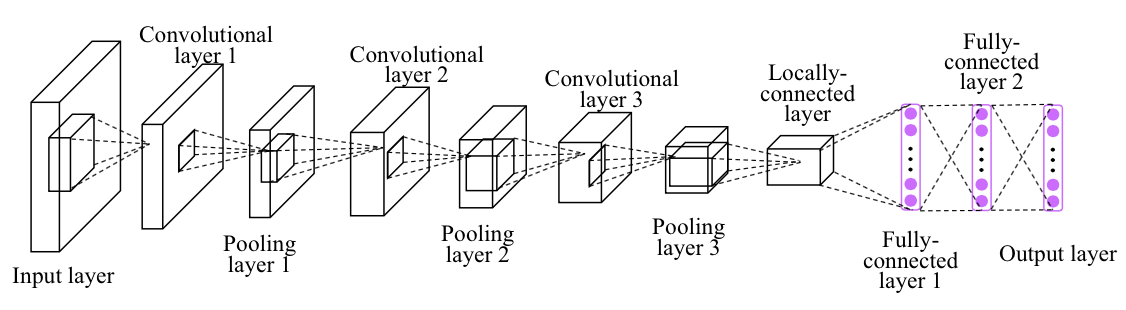
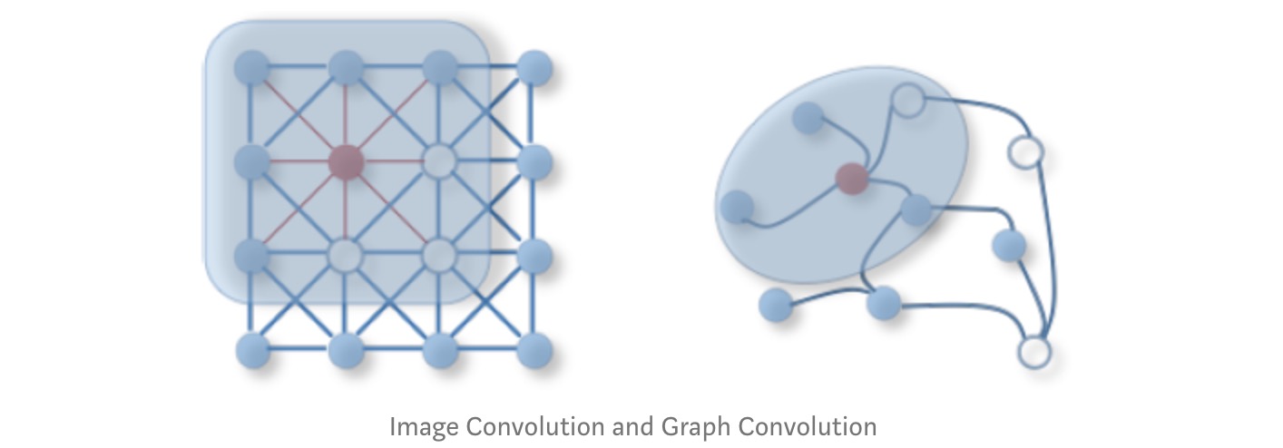
Recap: Convolutional Neural Networks (CNN)

• Local filter
• Translation invariance

source: Arden Dertat

Graph Neural Networks

Principles

• A deep learning framework for graph-structured data
• It generalises traditional neural networks to handle graph data by leveraging the relationships between nodes in a graph
• Message passing: nodes aggregate neighbor features over the graph
• Variants differ in how neighbors are aggregated and weighted

Major GNN Architectures

• GCN: shared filters; normalised neighborhood aggregation (spectral → spatial)
• GraphSAGE: inductive sampling + learnable aggregators (mean/pool/LSTM)
• GAT: attention over neighbors; learns edge weights; multi-head for capacity
• Not today’s focus, but worth mentioning
• DeepWalk: unsupervised node embeddings via random walks (word2vec-like)
• ChebNet: spectral filtering via Chebyshev polynomials; localised convolutions

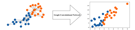
Graph Convolutional Networks (GCN)

Introduction: Graphs

• Graph = organised data representation
• Consists of vertices (nodes) V and edges E
• Edges can be weighted or binary
• Edges can be directed or undirected

Example graph:

\[V = \{A, B, C, D, E, F, G\}\] \[E = \{(A,B), (B,C), (C,E), ...\}\]

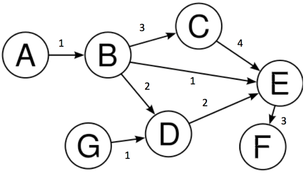
Graph Terminology

• Node: An entity in the graph (represented by circles)
• Edge: Line joining two nodes (represents relationships)
• Degree: Number of edges incident with a vertex
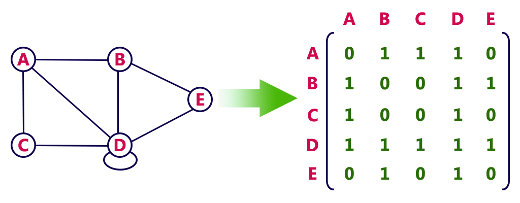
• Adjacency Matrix: N×N matrix representing graph structure

Why GCNs?

Why GCNs?

• Most real-world datasets come as graphs or networks:
  • Social networks
  • Protein-interaction networks
  • The World Wide Web
• Learning on graphs enables domain-specific insights
• Conventional CNNs assume compositional structure on Euclidean space
  • 2D grids (images)
  • 1D sequences (text, audio)

CNNs vs GCNs

CNN Key Properties:

• Locality
• Stationarity (Translation Invariance)
• Multi-scale hierarchies

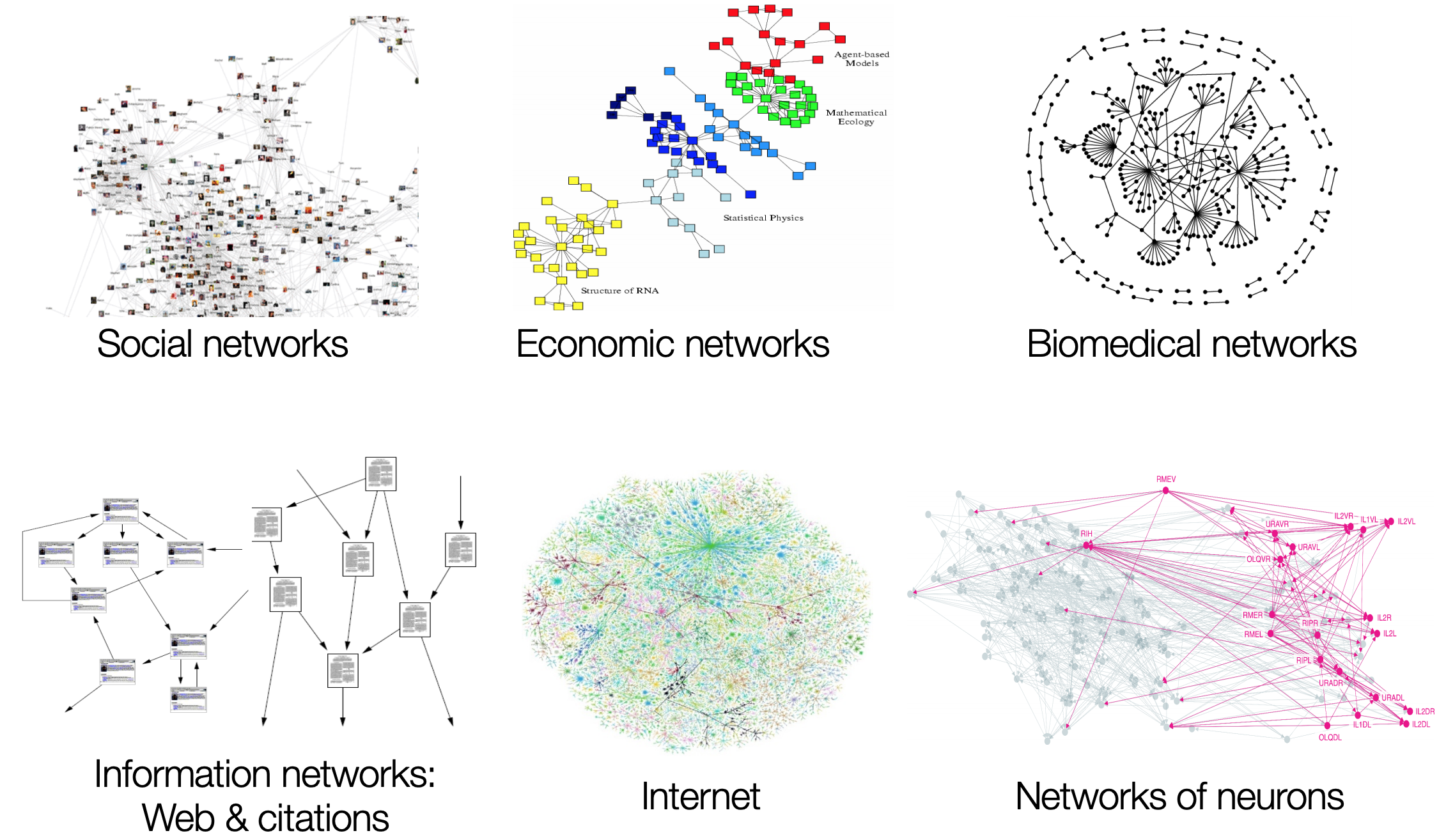
Problem: Not all data lies on Euclidean space!

Applications of GCNs

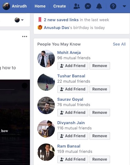
Facebook Link Prediction for Suggesting Friends using Social Networks

• Friend prediction algorithms
• Social network analysis
• Protein interaction prediction
• Knowledge graph completion

What are GCNs?

• Neural networks operating on graphs
• Capture neighbourhood information for non-euclidean spaces
• Re-define convolution for graph domains

Two Styles:

• Spectral GCNs: Graph signal processing perspective; Flourier transform on graphs; frequency domain
• Spatial GCNs: Aggregate feature information from neighbours; more flexible (OUR FOCUS!)

How GCNs Work? Friend Prediction

Task: Predict future friendships

• Edges = friendships
• More common friends → higher likelihood
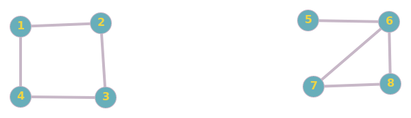
• \((1,3)\) have 2 common friends
• \((1,5)\) have 0 common friends
• So, \((1,3)\) is more likely to become friends than \((1,5)\)

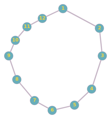
Try it again - Friend Prediction

Problem: Predict future friendships

• \((1,11)\) have 1 common friends and distance of 2
• \((3,11)\) have 0 common friends and distance of 4
• So, \((1,11)\) is more likely to become friends than \((3,11)\)

How to implement this idea MATHMATICALLY?

• Using filtering, from CNN?
• In CNN, we apply a filter on an image to get representation of next layer
• In a graph, we apply a filter to create the next layer representation, by aggregating the features of neighbours
• Note: in each layer, the graph structure is fixed, but the features of each node are updated.

Adjacency matrix & feature matrix

Adjacency matrix \[ A = \begin{pmatrix} 0 & 1 & 0 & 1 & 0 & 0 & 0 & 0 \\ 1 & 0 & 1 & 0 & 0 & 0 & 0 & 0 \\ 0 & 1 & 0 & 1 & 0 & 0 & 0 & 0 \\ 1 & 0 & 1 & 0 & 0 & 0 & 0 & 0 \\ 0 & 0 & 0 & 0 & 0 & 1 & 0 & 0 \\ 0 & 0 & 0 & 0 & 1 & 0 & 1 & 1 \\ 0 & 0 & 0 & 0 & 0 & 1 & 0 & 1 \\ 0 & 0 & 0 & 0 & 0 & 1 & 1 & 0 \end{pmatrix} \]

Feature matrix (Randomly initialised. Can be age, hobby, etc) \[ H^0 = \left( \begin{array}{ccc} 1 & 0 & 1 \\ 1 & 1 & 0 \\ 0 & 1 & 1 \\ 1 & 1 & 1 \\ 0 & 0 & 1 \\ 0 & 1 & 0 \\ 1 & 0 & 0 \\ 1 & 1 & 0 \end{array} \right) \]

Update rule for a node in a new layer

• Iteratively, calculate new features for each node in a new layer by aggregating from neighhours in the previous layer
• Each layer represent ‘friends’ information at different ‘hops’ \[ h_v^i = \sum_{u \in \mathcal{N}(v)} h_u^{i-1} \]

where \(\mathcal{N}(v)\) is the set of immediate neighbours of \(v\), excluding \(v\) itself.

Layer 1: \(H^1 = A H^0\)

• Node 1 (Neighbours: 2, 4):\(h_1^1 = h_2^0 + h_4^0 = [1, 1, 0] + [1, 1, 1] = \mathbf{[2, 2, 1]}\)
• Node 3 (Neighbours: 2, 4):\(h_3^1 = h_2^0 + h_4^0 = [1, 1, 0] + [1, 1, 1] = \mathbf{[2, 2, 1]}\)
• Node 5 (Neighbour: 6):\(h_5^1 = h_6^0 = \mathbf{[0, 1, 0]}\)
• Note: Node 1 and 3 have identifical features after one layer, due to same set of neighbours.
• \((1,3)\) is more similar than \((1,5)\)

Layer 2: \(H^2 = A H^1\). Friend-of-friend

• Node 1 (Neighbours: 2, 4):\(h_1^2 = h_2^1 + h_4^1 = [1, 1, 2] + [1, 1, 2] = \mathbf{[2, 2, 4]}\)
• Node 3 (Neighbours: 2, 4):\(h_3^2 = h_2^1 + h_4^1\)\(h_3^2 = [1, 1, 2] + [1, 1, 2] = \mathbf{[2, 2, 4]}\)
• Node 5 (Neighbour: 6):\(h_5^2 = h_6^1\)\(h_6^1 = h_5^0 + h_7^0 + h_8^0 = [2, 1, 1] = \mathbf{[2, 1, 1]}\)
• \((1,3)\) is more similar than \((1,5)\)

Convolution on a graph

Layer-wise propagation:

\[H^{i} = f(H^{i-1}, A)\]

\[f(H^{i}, A) = AH^{i}\]

where:

• \(A\) = N × N adjacency matrix
• \(H^{0} = X\) (initial features)
• \(X\) = input feature matrix (N × F, F = number of features)
• But: this formula is deterministic and linear, containing no learnable parameters
• To improve it, we introduce a non-linear ReLU activation function and a learnable weight matrix

GCN Mathematical Formulation

Layer-wise propagation:

\[H^{i} = f(H^{i-1}, A)\]

\[f(H^{i}, A) = σ(AH^{i}W^{i})\]

where:

• \(A\) = N × N adjacency matrix
• \(W^{(l)}\) = learnable weight matrix for layer \(l\). Shape \(F^{in}\) x \(F^{out}\).
  
• \(H^{0} = X\) (initial features), shape N × F
• \(X\) = input feature matrix (N × F, F = number of features)
• \(σ\) = ReLU activation function
• Each layer aggregates neighborhood features from previous layer

Problem 1: No self-representation

• New features don’t include node’s own features
• Node 1 and 3 become identical after one layer, despite different initial features
• Node 1 (Neighbours: 2, 4):\(h_1^1 = h_2^0 + h_4^0 = [1, 1, 0] + [1, 1, 1] = \mathbf{[2, 2, 1]}\)
• Node 3 (Neighbours: 2, 4):\(h_3^1 = h_2^0 + h_4^0 = [1, 1, 0] + [1, 1, 1] = \mathbf{[2, 2, 1]}\)

  

• Solution: Add self-loops
• Add identity: \(\hat{A} = A + I\)
• Node 1: \(h_1^1 = h_1^0 + h_2^0 + h_4^0 = [1,0,1] + [1,1,0] + [1,1,1] = \mathbf{[3, 2, 2]}\)
• Node 3: \(h_3^1 = h_2^0 + h_3^0 + h_4^0 = [1,1,0] + [0,1,1] + [1,1,1] = \mathbf{[2, 3, 2]}\)
• Now, they are different due to self-loops

Problem 2: Degree scaling

• High-degree nodes get larger values; low-degree nodes get smaller values
• Node 5 (Self + 6):\(h_5^1 = h_5^0 + h_6^0 = [0, 0, 1] + [0, 1, 0] = \mathbf{[0, 1, 1]}\)
• Node 6 (Self + 5, 7, 8):\(h_6^1 = h_6^0 + h_5^0 + h_7^0 + h_8^0 = [0, 1, 0] + [0, 0, 1] + [1, 0, 0] + [1, 1, 0] = \mathbf{[2, 2, 1]}\)

  

Problem 2: Degree scaling

• Solution: Normalise by degree
• Symmetric normalisation: \(\hat{D}^{-\frac{1}{2}}\hat{A}\hat{D}^{-\frac{1}{2}}\), where \(\hat{D}\) is degree matrix of \(\hat{A}\)
• \(\tilde{d}_5 = 2, \tilde{d}_6 = 4, \tilde{d}_7 = 3, \tilde{d}_8 = 3\)
• \(h_5^1 = \left( \frac{1}{\sqrt{\tilde{d}_5 \cdot \tilde{d}_5}} \right) h_5^0 + \left( \frac{1}{\sqrt{\tilde{d}_5 \cdot \tilde{d}_6}} \right) h_6^0 = \frac{1}{2}[0, 0, 1] + \frac{1}{\sqrt{8}}[0, 1, 0] \approx \mathbf{[0, 0.35, 0.5]}\)
• \(h_6^1 = 0.25[0, 1, 0] + 0.35[0, 0, 1] + 0.28[1, 0, 0] + 0.28[1, 1, 0] \approx \mathbf{[0.56, 0.53, 0.35]}\)

Final GCN Propagation Rule

\[f(H^{(l)}, A) = \sigma\left( \hat{D}^{-\frac{1}{2}}\hat{A}\hat{D}^{-\frac{1}{2}}H^{(l)}W^{(l)}\right)\]

where:

• \(\hat{A} = A + I\) (adjacency + self-loops)
• \(I\) = identity matrix
• \(\hat{D}\) = diagonal degree matrix of \(\hat{A}\)
• \(W^{(l)}\) = learnable weight matrix for layer \(l\)
• \(\sigma\) = activation function

Implementing GCN in PyTorch

GCN Convolutional Layer

class GCNConv(nn.Module):
    def __init__(self, A, in_channels, out_channels):
        super(GCNConv, self).__init__()
        self.A_hat = A + torch.eye(A.size(0))
        self.D     = torch.diag(torch.sum(A,1))
        self.D     = self.D.inverse().sqrt()
        self.A_hat = torch.mm(torch.mm(self.D, self.A_hat), self.D)
        self.W     = nn.Parameter(torch.rand(in_channels,out_channels))
    
    def forward(self, X):
        out = torch.relu(torch.mm(torch.mm(self.A_hat, X), self.W))
        return out

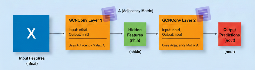
GCN Network Architecture

class Net(torch.nn.Module):
    def __init__(self, A, nfeat, nhid, nout):
        super(Net, self).__init__()
        self.conv1 = GCNConv(A, nfeat, nhid)
        self.conv2 = GCNConv(A, nhid, nout)
        
    def forward(self, X):
        H  = self.conv1(X)
        H2 = self.conv2(H)
        return H2

Case Study: Zachary’s Karate Club

Context (1970-1972):

• Observed local karate club
• Conflict between administrator “John A” and instructor “Mr. Hi” led to club split into two groups
• Based on this graph, aim to predict which members join which group

Semi-Supervised Learning Setup

• Labels known for only 2 nodes: John A (0) and Mr. Hi (1)
• Predict labels for all other members based on graph structure
• Use graph connectivity to propagate information

# Only nodes 0 and 33 are labeled
target = torch.tensor([0,-1,-1,-1,...,-1,-1,1])

# Feature matrix (one-hot encoding)
X = torch.eye(A.size(0))

# 'A' is the adjacency matrix of the karate club graph. It contains 1 at position (i,j) if there is an edge between node i and j, and 0 otherwise.

Training the Model

X=torch.eye(A.size(0))  # Identity matrix as initial X features

# Here we are creating a network with 10 features in hidden layer and 2 in output layer (John A's group vs Mr. Hi's group)

# Initialise network
model = Net(A, X.size(0), 10, 2)

# Loss and optimizer
criterion = torch.nn.CrossEntropyLoss(ignore_index=-1)
optimizer = optim.SGD(model.parameters(), lr=0.01, momentum=0.9)

# Training loop
for epoch in range(200):
    optimizer.zero_grad()
    loss = criterion(model(X), target)
    loss.backward()
    optimizer.step()

Training the model

• What parameters are trained? Weight matrix W and a bias vector for each layer (intercept)
  • Layer 1 (conv1): A matrix of size (nfeat, nhid)
  • Layer 2 (conv2): A matrix of size (nhid, nout)

\[f(H^{(l)}, A) = \sigma\left( \hat{D}^{-\frac{1}{2}}\hat{A}\hat{D}^{-\frac{1}{2}}H^{(l)}W^{(l)}\right)\]

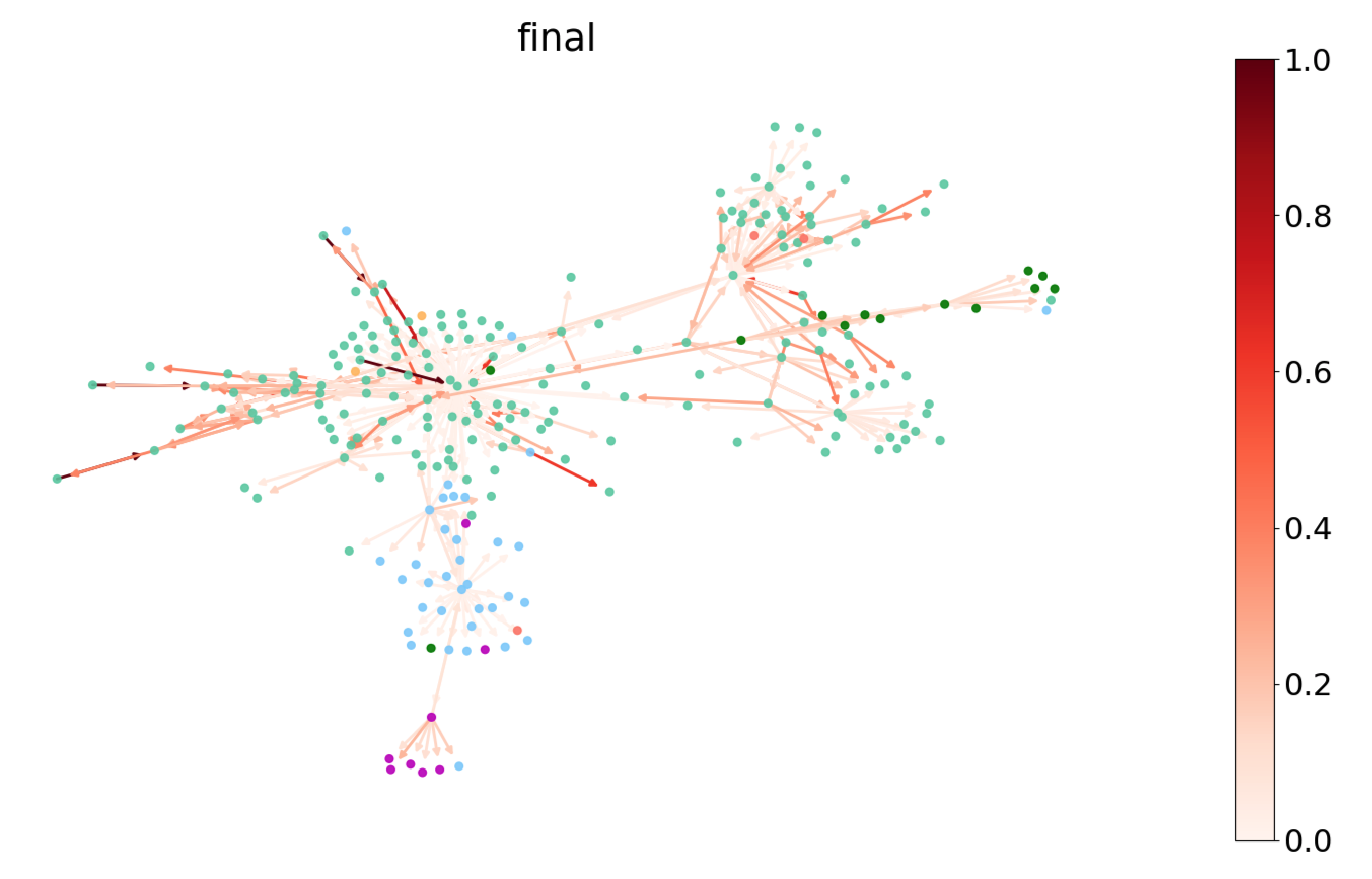
Training Visualisation

Node embeddings learned during training

• Model successfully separates two groups
• Close to actual predictions (except node 9)
• Semi-supervised learning works!

PyTorch Geometric

PyTorch Geometric (PyG):

• Dedicated library for graph deep learning
• Easy, fast, and simple implementation
• Active development and community

Features:

• Pre-built GCN layers
• Various graph datasets
• Efficient sparse operations

from torch_geometric.nn import GCNConv

class GCN(torch.nn.Module):
    def __init__(self):
        super().__init__()
        self.conv1 = GCNConv(num_features, 16)
        self.conv2 = GCNConv(16, num_classes)
        
    def forward(self, x, edge_index):
        x = self.conv1(x, edge_index)
        x = F.relu(x)
        x = self.conv2(x, edge_index)
        return F.log_softmax(x, dim=1)

GraphSAGE

Why GraphSAGE (Sample and Aggregate)?

• GCNs are transductive: requires full graph structure; can’t generalise to unseen nodes/graphs
• GraphSAGE is inductive: learns aggregation functions that can be applied to unseen nodes/graphs

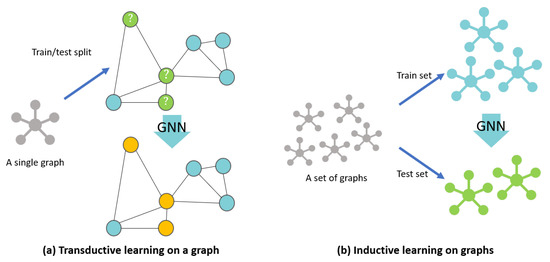
Transductive vs inductive learning on graph. Source: https://www.mdpi.com/2220-9964/10/2/97

Why GraphSAGE (Sample and Aggregate)?

• GraphSAGE is more scalable: neighborhood sampling to generate mini-batches, rather than processing the entire graph at once
• GraphSAGE allows for learnable aggregators: mean, pooling (MLP + max), LSTM; where GCN uses fixed mean aggregation
• GraphSAGE learns weights per layer; where GCN uses fixed weights from adjacency matrix
• GraphSAGE treats self-representation and neighbours differently: concatenating.

GraphSAGE Aggregators

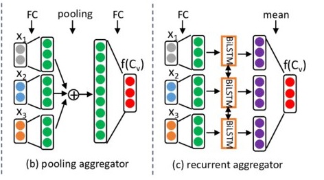
• Mean aggregator: elementwise mean over neighbors
• Pool aggregator: transform neighbor features using a MLP, then max-pool
• LSTM aggregator: sequence model over randomly ordered neighbors

Example of GraphSAGE update rules

• Step 1: Initial Features (\(H^0\))
• Node 6: \(h_6^0 = [0, 1]\)
• Neighbours (5, 7, 8): \(h_5^0 = [0, 0]\), \(h_7^0 = [1, 0]\), \(h_8^0 = [1, 1]\)

Step 2: Aggregate the Neighbours

\[\text{AGG}_{\text{neigh}} = \text{mean}([0, 0], [1, 0], [1, 1]) = [0.66, 0.33]\]

Step 3: Concatenation

• Join the self-vector and the neighbour-vector (increase dimension from 2 to 4) \[\text{CONCAT}(h_6^0, \text{AGG}_{neigh}) = [ \underbrace{0, 1}_{\text{Self}}, \underbrace{0.66, 0.33}_{\text{Neighbours}} ]\]

Step 4: Linear Transformation (\(W^k\))

• Bring the dimension back, from 4 to 2
• Suppose \(W^1\) is a \(2 \times 4\) matrix \[h_6^1 = \sigma \left( \begin{pmatrix} w_{11} & w_{12} & w_{13} & w_{14} \\ w_{21} & w_{22} & w_{23} & w_{24} \end{pmatrix} \cdot \begin{bmatrix} 0 \\ 1 \\ 0.66 \\ 0.33 \end{bmatrix} \right)\]

Why concatenation works?

• Identity Preservation: in GCN, if Node 6 has 100 neighbours, its own features only contribute \(1\%\) to the next layer. In GraphSAGE, the self-features always occupy a dedicated portion of the input to the next layer (as the first half of the concat vector).
• Flexible Weighting: weight matrix \(W\) can learn to weight “self” differently than “neighbours”.
  • Note: \(W\) is learned per layer from training, not fixed.
  • It might learn that your own interests are more important for friend prediction than your neighbours’ interests.

When to use GCN or GraphSAGE?

• Use GCN for small, static, or fully known graphs where node information does not change rapidly.
• Use GraphSAGE for large, dynamic, or streaming graphs, where you need to generate embeddings for unseen or new nodes without retraining the entire model.

Graph Attention Networks (GAT)

Why GAT?

• Treating neighhours differently: GCN use fixed aggregation (mean, sum, etc.) that treats all neighbors equally. GAT learns to assign different importance to different neighbors using attention mechanisms.
• Weight Calculation: GCN uses fixed, structural weights (based on graph Laplacian). GAT learns these weights dynamically during training
• Better Performance: GAT generally outperforms GCN on node classification task. GATs are particularly effective when the graph structure is complex or sparse.
• Higher Computational Complexity: GAT is more resource-intensive and slower to train; GCN is faster and more situable for large-scale graphs.

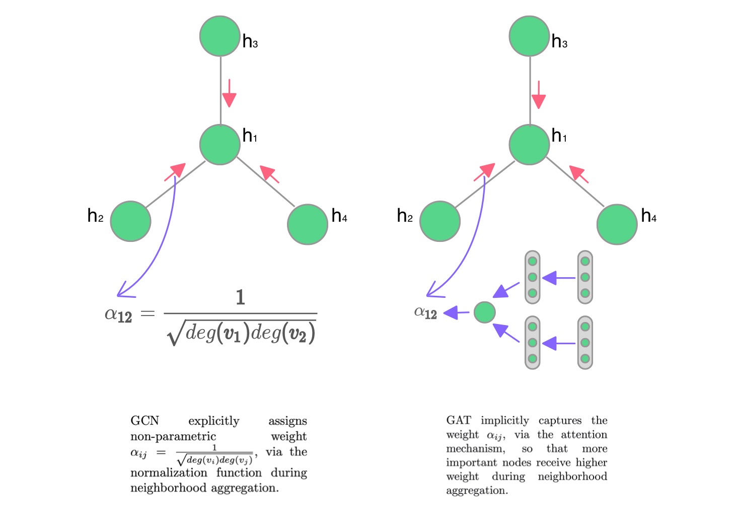
What is ATTENTION in GAT?

• Attention weight \(\alpha_{i,j}\) measures the importance of neighbor \(j\) to node \(i\)

\(h_i^{(l+1)} = \sigma \left( \sum_{j \in \mathcal{N}_i} \alpha_{ij}^{(l)} \mathbf{W}^{(l)} h_j^{(l)} \right)\)

Attention weight

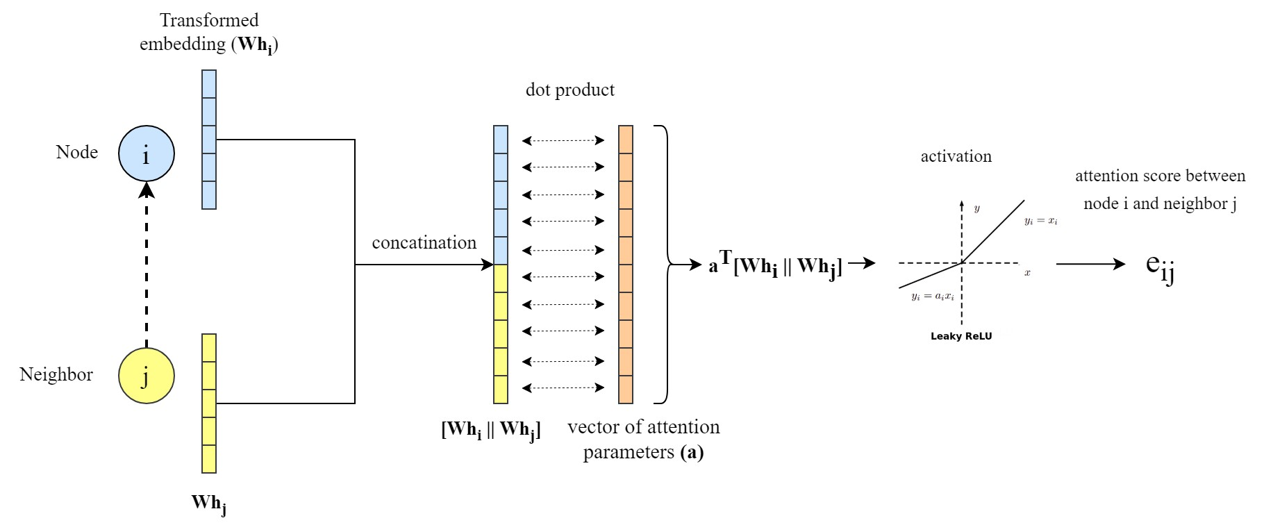
• A clear explanation: https://epichka.com/blog/2023/gat-paper-explained/

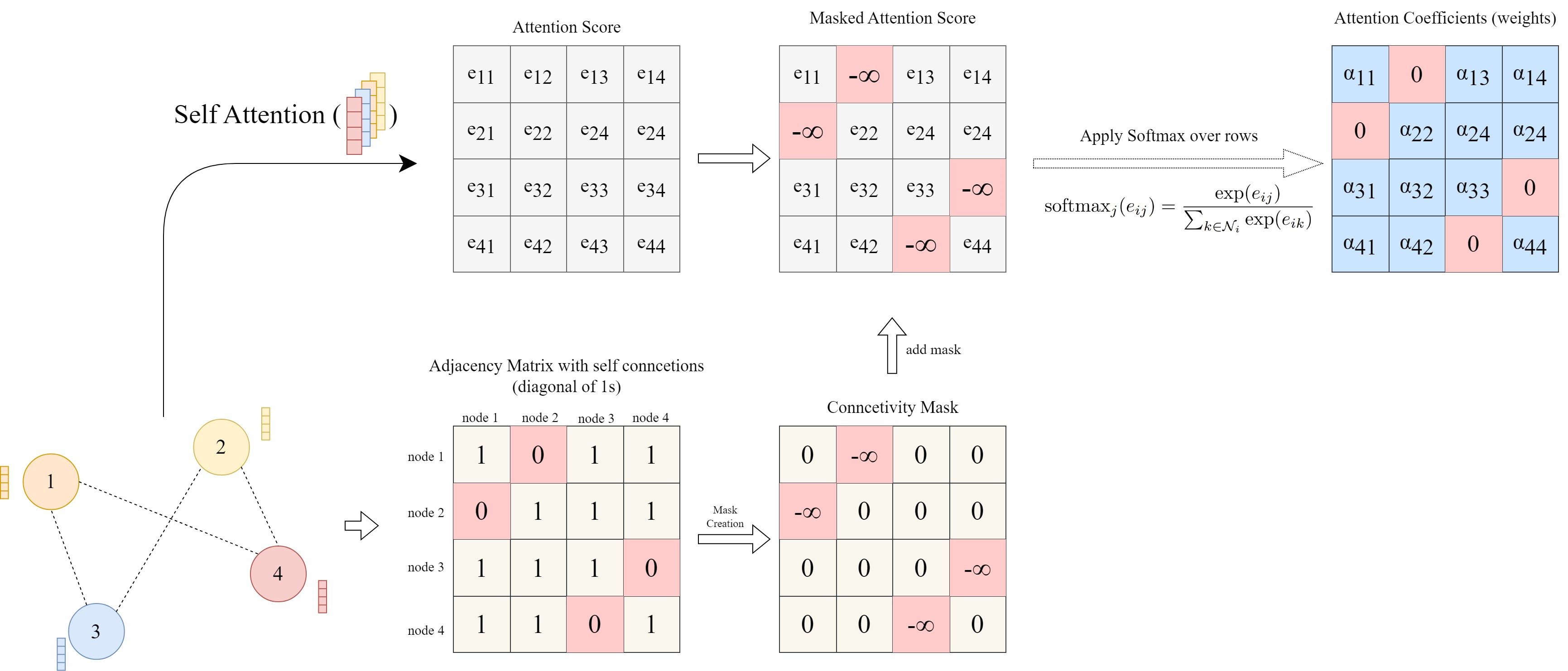
Masked Attention

• Only weights for neighbors are computed, others masked

Multi-head Attention to stabilise learning

• To mitigate randomness in calculating attention weights, e.g. random initialisation

\[h_i^{(l+1)} = \sigma \left( \frac{1}{K} \sum_{k=1}^{K} \sum_{j \in \mathcal{N}_i} \alpha_{ij}^{k} \mathbf{W}^{k} h_j^{(l)} \right)\]

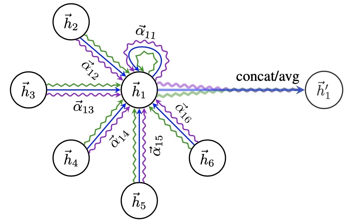
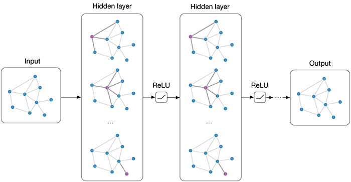
Concatenate intermediate heads; average at final layer

Attention visualisation for interpretability

• To understand which neighbors are most influential for a node

https://www.dgl.ai/blog/2019/02/17/gat.html

Key Takeaways

• GCNs extend neural networks to non-Euclidean graph data
• Aggregate and transform neighbourhood information
• Address self-representation and degree scaling issues
• Semi-supervised learning on graphs is powerful
• Applications: social networks, molecules, knowledge graphs

Q: How powerful are GCNs really?

Read: How powerful are Graph Convolutions?

Resources

• graphnet Github repo

Key Papers:

• Semi-Supervised Classification with GCNs - Kipf & Welling (2017)
• Thomas Kipf’s Blog on GCNs

Libraries:

• PyTorch Geometric
• Deep Graph Library (DGL)

Questions?