Neural Networks

Feed-Forward Networks and Deep Learning

Huanfa Chen - huanfa.chen@ucl.ac.uk

09/02/2026

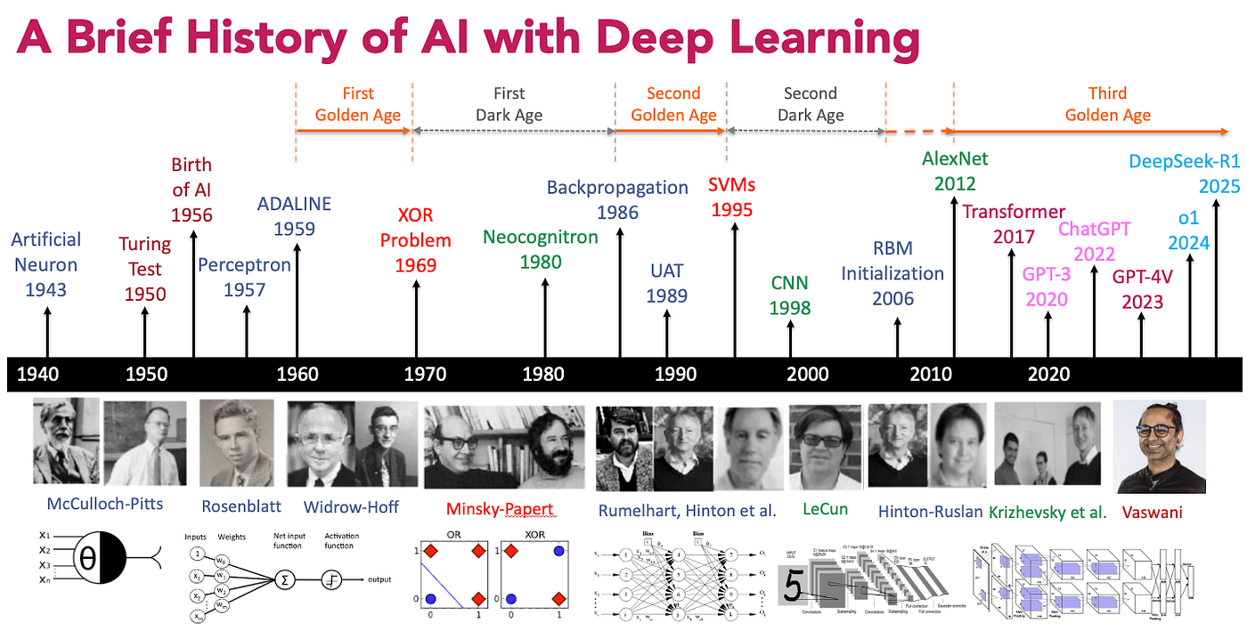
History

Image Credit: medium.com

History

• Nearly everything we talk about today existed in 1990
• What changed since then?
  • More data
  • Faster computers (GPUs)
  • Some improvements: Relu, dropout, adam, batch-normalization, residual networks

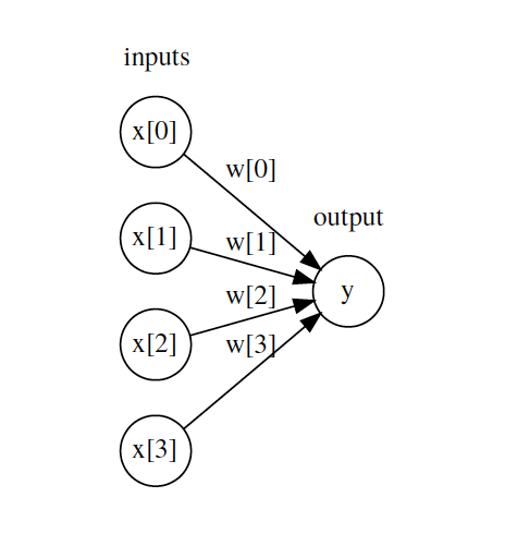
Linear Regression as Neural Net

\(y = \sum_i W_i x_i + b = Wx + b\)

\(y = g(Wx + b)\), where \(g(z) = z\) (identity function)

Logistic Regression as Neural Net

\(y = \sigma(Wx + b)\)

\(\sigma(z) = \frac{1}{1 + e^{-z}}\)

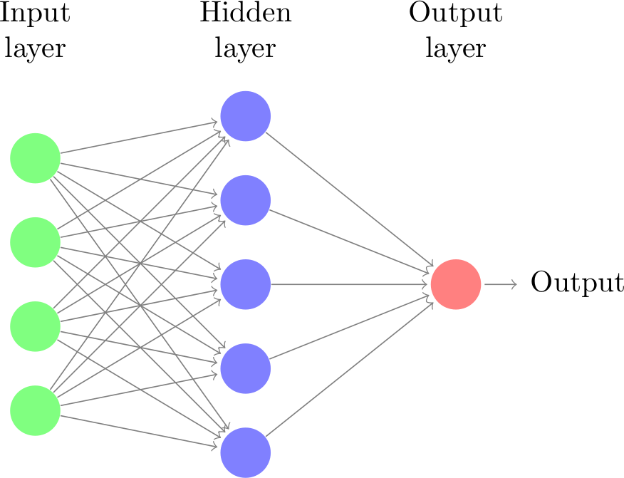
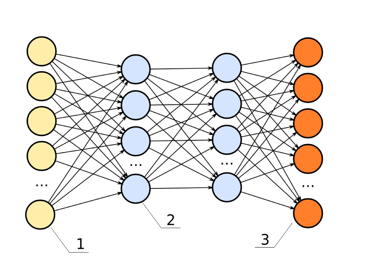
Basic Architecture of Neural Networks

\(h(x) = f(W_1x + b_1)\); f: hidden layer activation function

\(o(x) = g(W_2h(x) + b_2)\) g: output layer activation function

Output layer activation function \(g\)

• For regression: \(g\) is identity function \(g(z) = z\)
• For binary classification: \(g\) is sigmoid function \(g(z) = \sigma(z)\) (to output a probability [0,1])
• For multi-class classification: \(g\) is softmax function \(g(z_i) = \frac{e^{z_i}}{\sum_j e^{z_j}}\) (to output a probability distribution over classes)

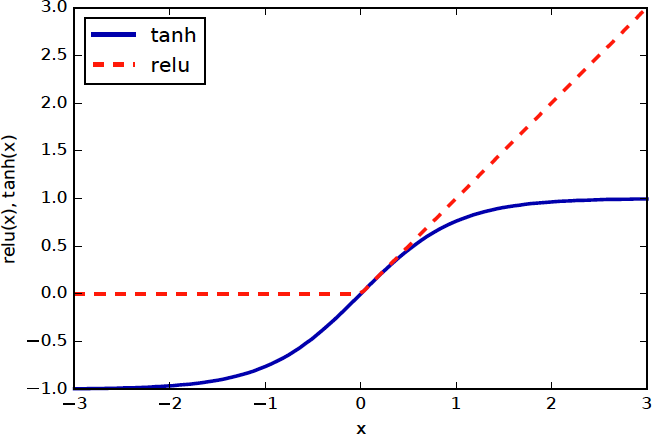
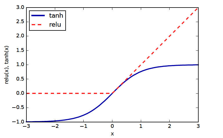
Nonlinear Activation Functions \(f\)

• The primary job of f is to break the linearity of the model
• Standard choices: tanh (pronounced like “than”) or relu (rectified linear unit) (pronounced as /ray-loo/)
• Tanh squashes between -1 and 1; saturates towards infinities
• ReLU is constant zero for negative numbers, then identity

More Layers

• Hidden layers usually all have the same non-linear function
• Other names: Multilayer perceptron, feed-forward neural network
• Many layers → “deep learning”

Supervised Neural Networks

• Non-linear models for classification and regression
• Work well for very large datasets
• Notoriously slow to train; need for GPUs
• Use dot products \(Wx\); require preprocessing similar to SVM or PCA, unlike trees
• Many variants: Convolutional nets, GRUs, LSTMs, recursive networks, VAEs, GANs, deep RL

Training Objective

\(h(x) = f(W_1x+b_1)\)

\(o(x) = g(W_2h(x)+b_2) = g(W_2f(W_1x + b_1) + b_2)\)

• The objective is to minimise the difference between true and predicted y values, or the loss function

\(\min_{W_1,W_2,b_1,b_2} \sum\limits_{i=1}^N l(y_i,o(x_i))\)

\(= \min_{W_1,W_2,b_1,b_2} \sum\limits_{i=1}^N l(y_i,g(W_2f(W_1x+b_1)+b_2))\)

• \(l\) = Squared loss for regression; Cross-entropy loss for classification

Backpropagation

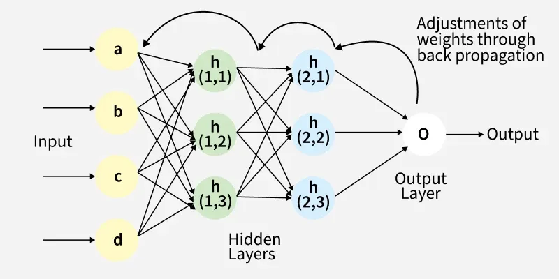
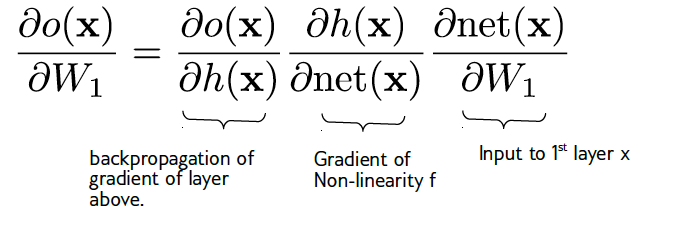
Backpropagation

• Need \(\frac{\partial l(y, o)}{\partial W_i}\) and \(\frac{\partial l(y, o)}{\partial b_i}\)

\(\text{net}(x) := W_1x + b_1\)

Gradient Computation

• Backpropagation is clever application of chain rule for derivatives
• Single backward pass from output to input computes derivatives
• An efficient way to compute gradients
• Training NN is an optimisation problem, which means to find the optimal parameters \(W_i\) and \(b_i\) that minimise the loss function
• Training NN is a non-convex and challenging optimisation problem. Usually a local optimum is found.

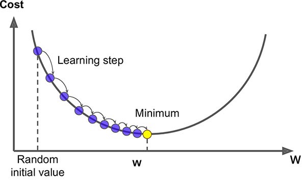
Recap on gradient

• Optimise \(\arg\min_w F(w)\) by stepping along \(-\nabla F(w)\)
• Update: \(w_{i+1} = w_i - \eta_i \nabla F(w_i)\)
• Converges to a local minimum

ReLU Differentiability

• ReLU not differentiable at zero. At x>0, gradient is 1; at x<0, gradient is 0
• For a function to be differentiable, the slope must be the same whether approaching from the left or right
• Use subgradient descent; any gradient below the function works
• In practice, most FL framewors simply hardcode the gradient at zero to be 0 or 0.5

Optimising W, b

Usually, We don’t use all data to compute the gradient at each step.

Batch \(W_i \leftarrow W_i - \eta\sum\limits_{j=1}^N \frac{\partial l(x_j,y_j)}{\partial W_i}\)

Instead, we can use a subset of data to estimate the gradient.

Online/Stochastic \(W_i \leftarrow W_i - \eta\frac{\partial l(x_j,y_j)}{\partial W_i}\)

Minibatch \(W_i \leftarrow W_i - \eta\sum\limits_{j=k}^{k+m} \frac{\partial l(x_j,y_j)}{\partial W_i}\)

Learning Heuristics

• \(\eta\) controls the step size of gradient descent. Can adjust during training.
• Constant \(\eta\) is not good
• Can decrease \(\eta\) over time
• Better: adaptive \(\eta\) for each entry of \(W_i\)
• State-of-the-art: Adam (Adaptive Moment Estimation)

Adam optimiser

• The logic: for a parameter, if a gradient is consistely large, should decrease the learning rate and slow down;
• If a gradient is consistely small, should increase the learning rate for that parameter.
• The process: keep track of the first moment (mean) and second moment (uncentered variance) of the gradients; use them to adapt the learning rate for each parameter

Update rule of Adam optimiser

1. Estimate 1st moment: \(m_t = \beta_1 m_{t-1} + (1 - \beta_1)g_t\)
2. Estimate 2nd moment: \(v_t = \beta_2 v_{t-1} + (1 - \beta_2)g_t^2\)
3. Bias Correction: as \(m_t\) and \(v_t\) start at zero, Adam uses a mathematical trick to “warm them up” during the first few steps.
4. Update Weight: \(\theta_{t+1} = \theta_t - \frac{\eta}{\sqrt{\hat{v}_t} + \epsilon} \hat{m}_t\)

Picking Optimisation Algorithms

• Small dataset: off-the-shelf like l-bfgs (quicker than Adam on small datasets)
• Big dataset: adam / rmsprop
• Have time & nerve: tune the schedule

Neural Nets with sklearn

mlp = MLPClassifier(solver='lbfgs', random_state=0).fit(X_train, y_train)
print(mlp.score(X_train, y_train))
print(mlp.score(X_test, y_test))

• Don’t use sklearn for real projects but toy problems in neural nets
• Why? sklearn’s MLP is not optimised for large datasets; no GPU support; no support for conv nets, etc.

Complexity Control

• Number of parameters: hidden layers, hidden units
• Regularisation
• Early Stopping
• Dropout

NN subject to overfitting and random seeds

• Network is way over capacity and can overfit in many ways
• Regularisation might make it less dependent on initialization

Regularisation

• Regularisation works by modifying the loss function: \(L = \sum\limits_{i=1}^N l(y_i, o(x_i))\)
• L2 regularisation: add \(\lambda \sum\limits_i W_i^2\) to loss function; to penalise large weights
• L1 regularisation: add \(\lambda \sum\limits_i |W_i|\) to loss function; to encourage many weights to be zero
• Dropout: randomly set some activations to zero during training; prevents co-adaptation of neurons

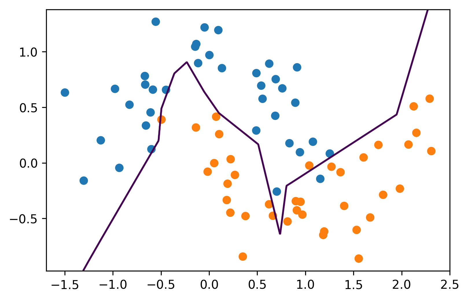
Hidden Layer Size

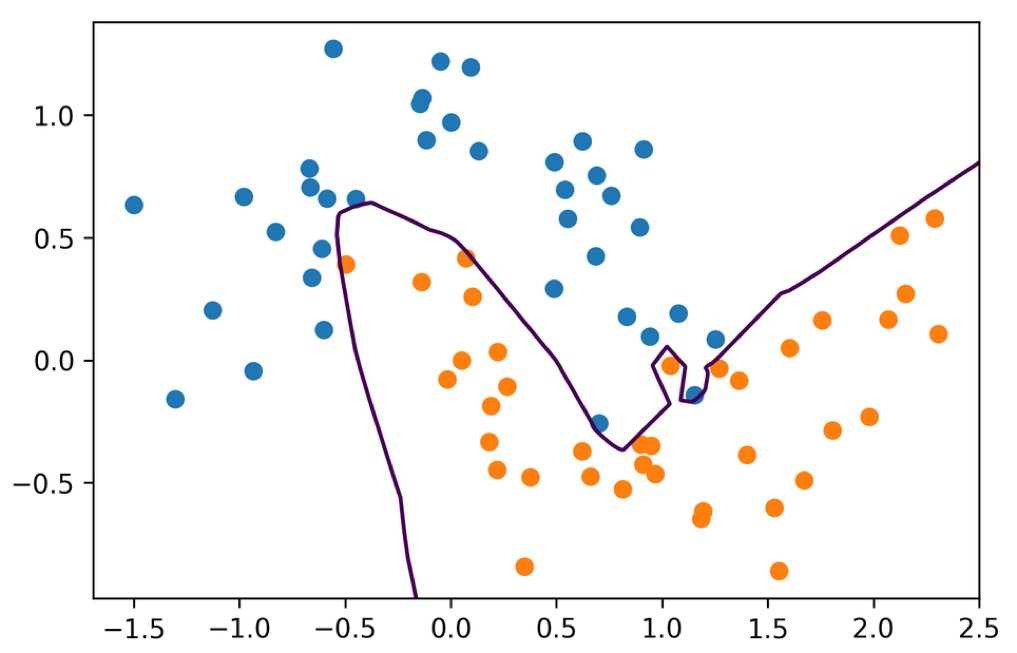
mlp = MLPClassifier(solver='lbfgs', hidden_layer_sizes=(5,), random_state=10)
mlp.fit(X_train, y_train)

• Single hidden layer with 5 units
• Each unit corresponds to different part of decision boundary

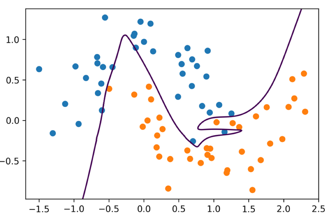
Multiple Hidden Layers

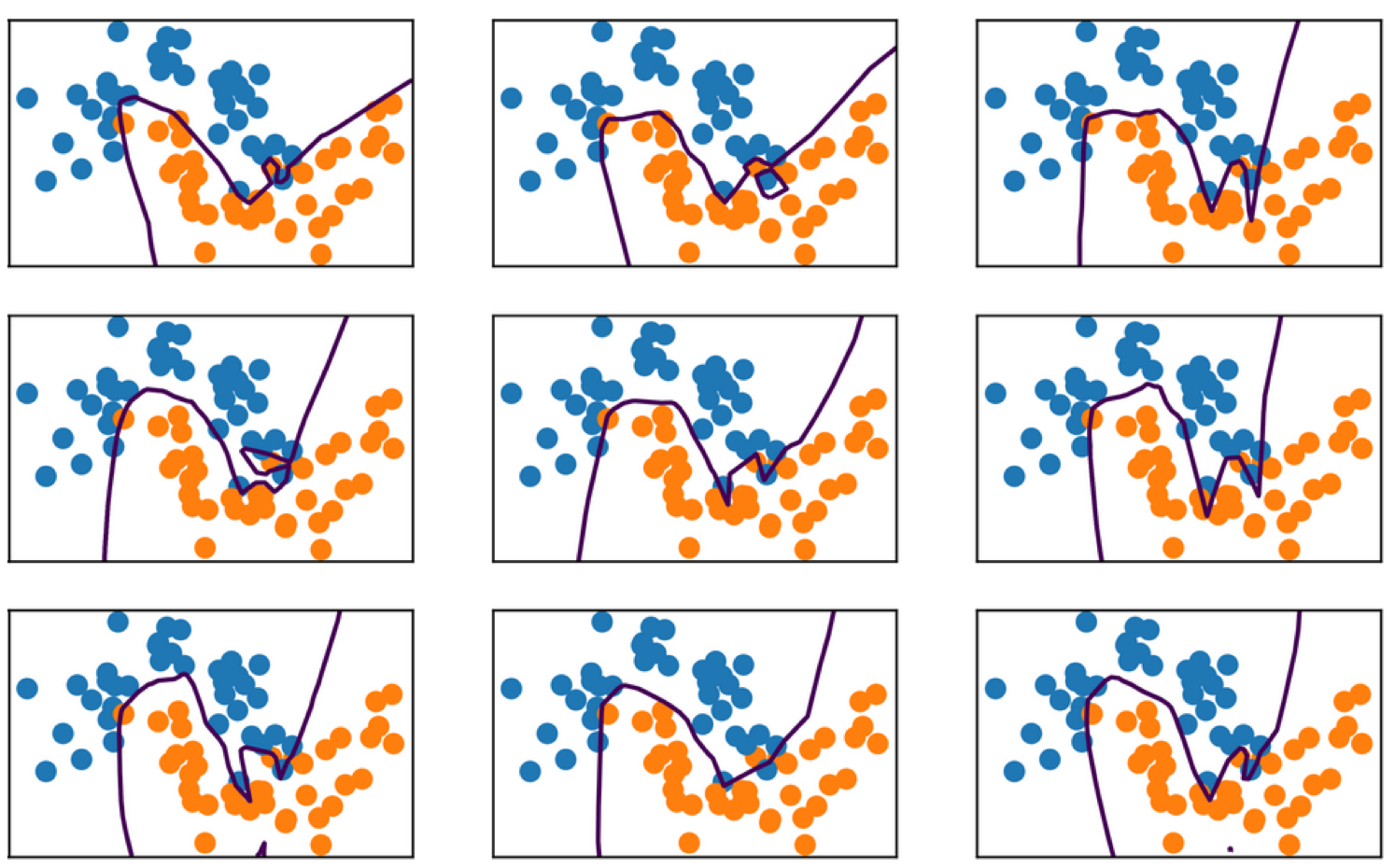
mlp = MLPClassifier(solver='lbfgs', hidden_layer_sizes=(10, 10, 10), random_state=0)
mlp.fit(X_train, y_train)

• 3 hidden layers each of size 10
• Main way to control complexity

Activation Functions

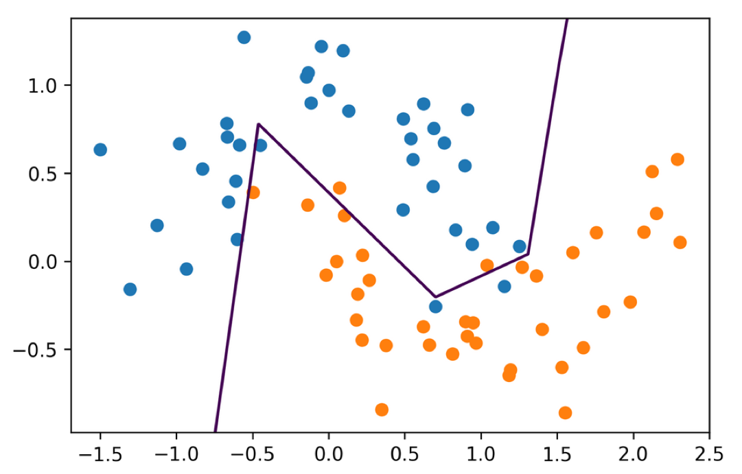
mlp = MLPClassifier(solver='lbfgs', hidden_layer_sizes=(10, 10, 10),
                    activation='tanh', random_state=0)
mlp.fit(X_train, y_train)

• Using tanh gives smoother boundaries
• ReLU doesn’t work as well with l-bfgs on small networks
• For large networks, relu is preferred

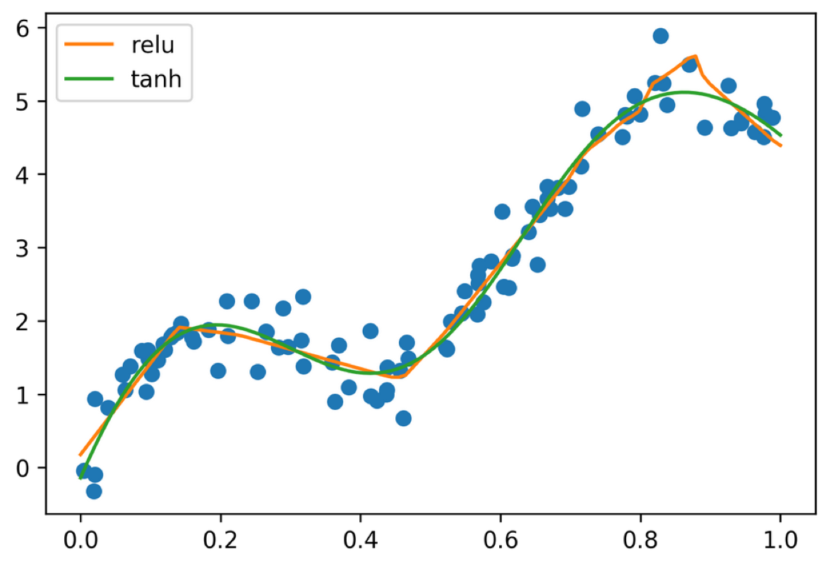
Regression

from sklearn.neural_network import MLPRegressor
mlp_relu = MLPRegressor(solver=\"lbfgs\").fit(X, y)
mlp_tanh = MLPRegressor(solver=\"lbfgs\", activation='tanh').fit(X, y)

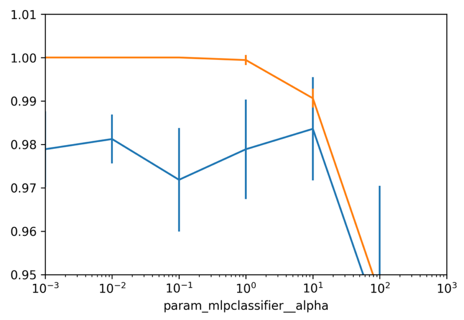
Grid-Searching Neural Nets

from sklearn.datasets import load_breast_cancer
data = load_breast_cancer()
X_train, X_test, y_train, y_test = train_test_split(
    data.data, data.target, stratify=data.target, random_state=0)

from sklearn.model_selection import GridSearchCV
pipe = make_pipeline(StandardScaler(), MLPClassifier(solver=\"lbfgs\", random_state=1))
param_grid = {'mlpclassifier__alpha': np.logspace(-3, 3, 7)}
grid = GridSearchCV(pipe, param_grid)

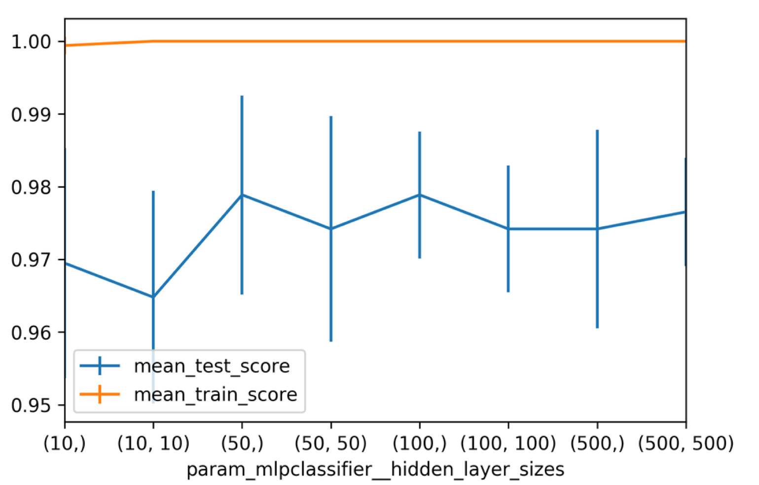
Searching Hidden Layer Sizes

from sklearn.model_selection import GridSearchCV
pipe = make_pipeline(StandardScaler(), MLPClassifier(solver=\"lbfgs\", random_state=1))
param_grid = {'mlpclassifier__hidden_layer_sizes':
              [(10,), (50,), (100,), (500,), (10, 10), (50, 50), (100, 100), (500, 500)]}
grid = GridSearchCV(pipe, param_grid)
grid.fit(X_train, y_train)

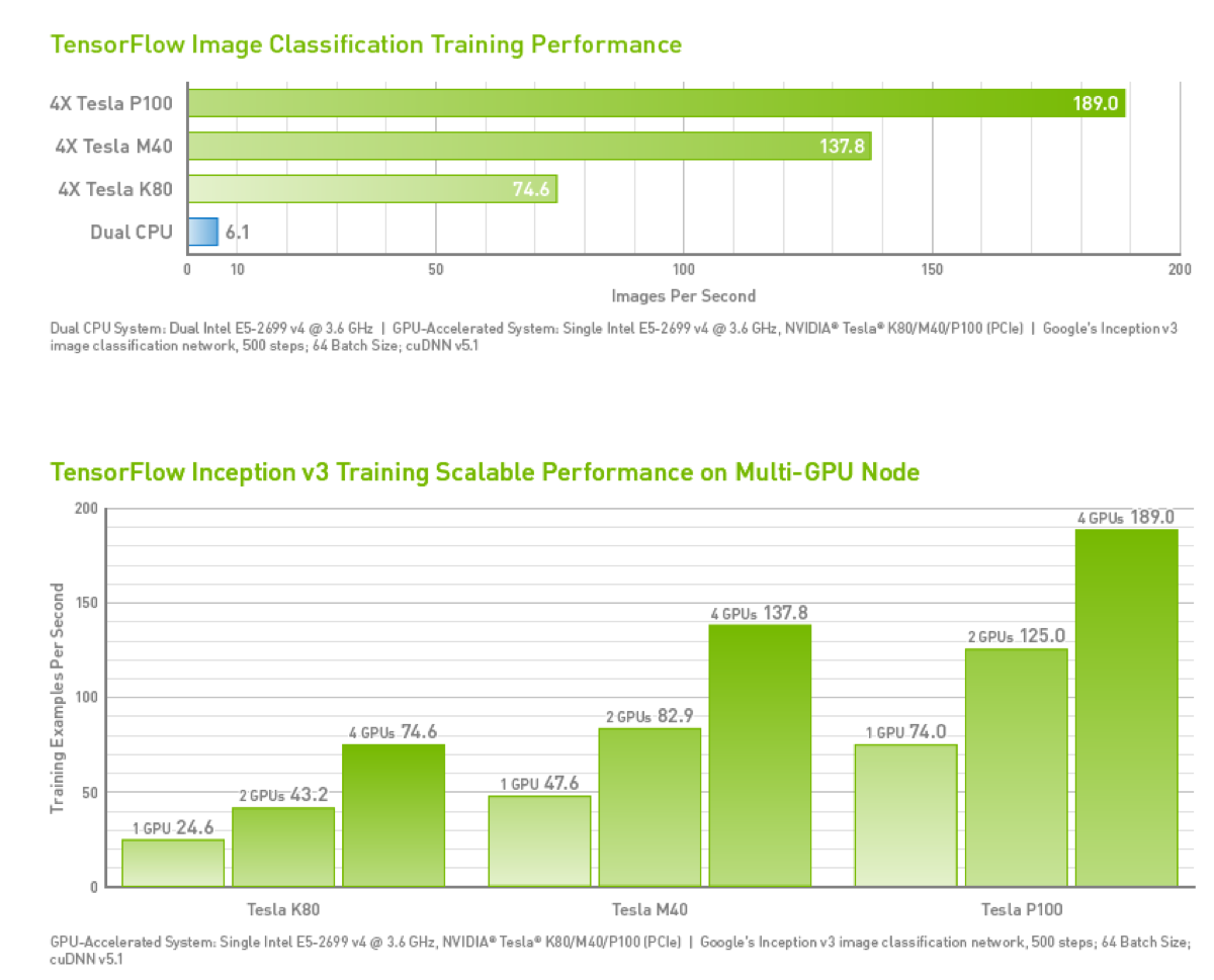
GPU Support

• Important limitation: GPUs have much less memory than RAM
• Memory copies between RAM and GPU are expensive

CPU VS. GPU

Feature	CPU	GPU
Architecture	Few cores optimised for sequential tasks	Thousands of cores for parallel processing
Memory	Larger cache size, less memory bandwidth	Higher memory bandwidth, less cache size
Power Consumption	Generally lower power consumption	Higher power consumption due to many cores
Use Cases	General-purpose computing, complex logic	Graphics rendering, deep learning, scientific simulations
Cost	Less expensive	Expensive
Programming Complexity	Easier to program for general tasks	Requires knowledge of parallel programming (e.g., CUDA)

How much GPU power do you need?

Task Type	Typical GPU	Total GPU Hours	Estimated Cost (Cloud)
Small Project (MNIST, basic CNN)	1x RTX 3060 / 4060	< 1 hour	< $1
Fine-tuning 7B LLM (e.g., Llama 3 8B)	1x A100 (80GB)	5–20 hours	$10 – $40
Training Mid-size Model (e.g., Stable Diffusion)	8x A100 Cluster	500–2,000 hours	$1,000 – $5,000
Pre-training Large LLM (GPT-3/4 scale)	10,000+ H100s	Millions of hours	$50M – $100M+

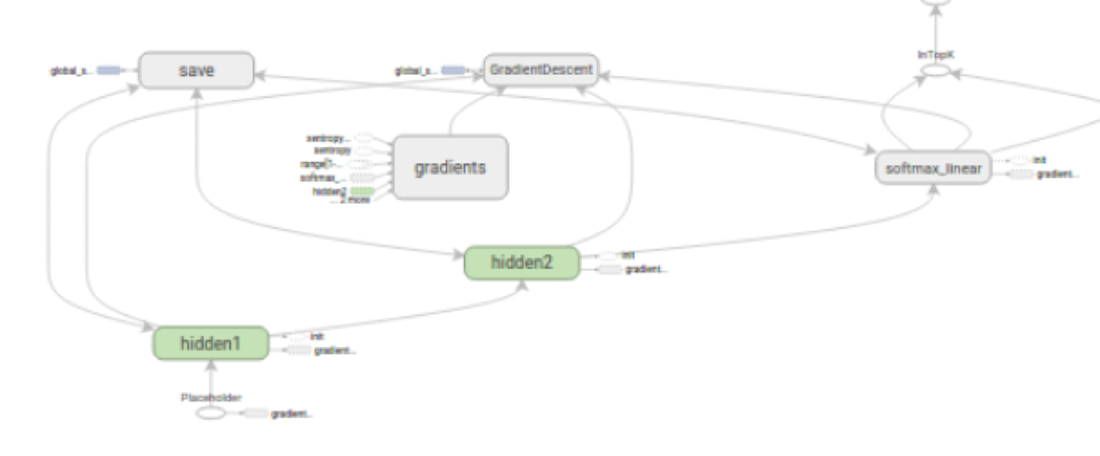
Computational Graph

• ‘blue-print’; a directed acyclic graph representing computations in NN
• Nodes represent variables or operations (e.g., matrix multiplication, activation functions), edges represent flow of data (tensors) between operations
• Given limited GPU memory, important to know what to cache/discard
• Helps with visual debugging and understanding network structure

Deep Learning Framework Requirements

• Autodiff
• GPU support
• Optimisation and inspection of computation graph
• On-the-fly generation of computation graph (optional)
• Distribution over multiple GPUs and/or cluster (optional)

Current choices: PyTorch / Torch, TensorFlow

Deep Learning Libraries

• PyTorch (torch) (default for AI research & development)
• Keras (TensorFlow, CNTK, Theano) (enterprise production)
• Chainer (chainer)
• MXNet (MXNet)

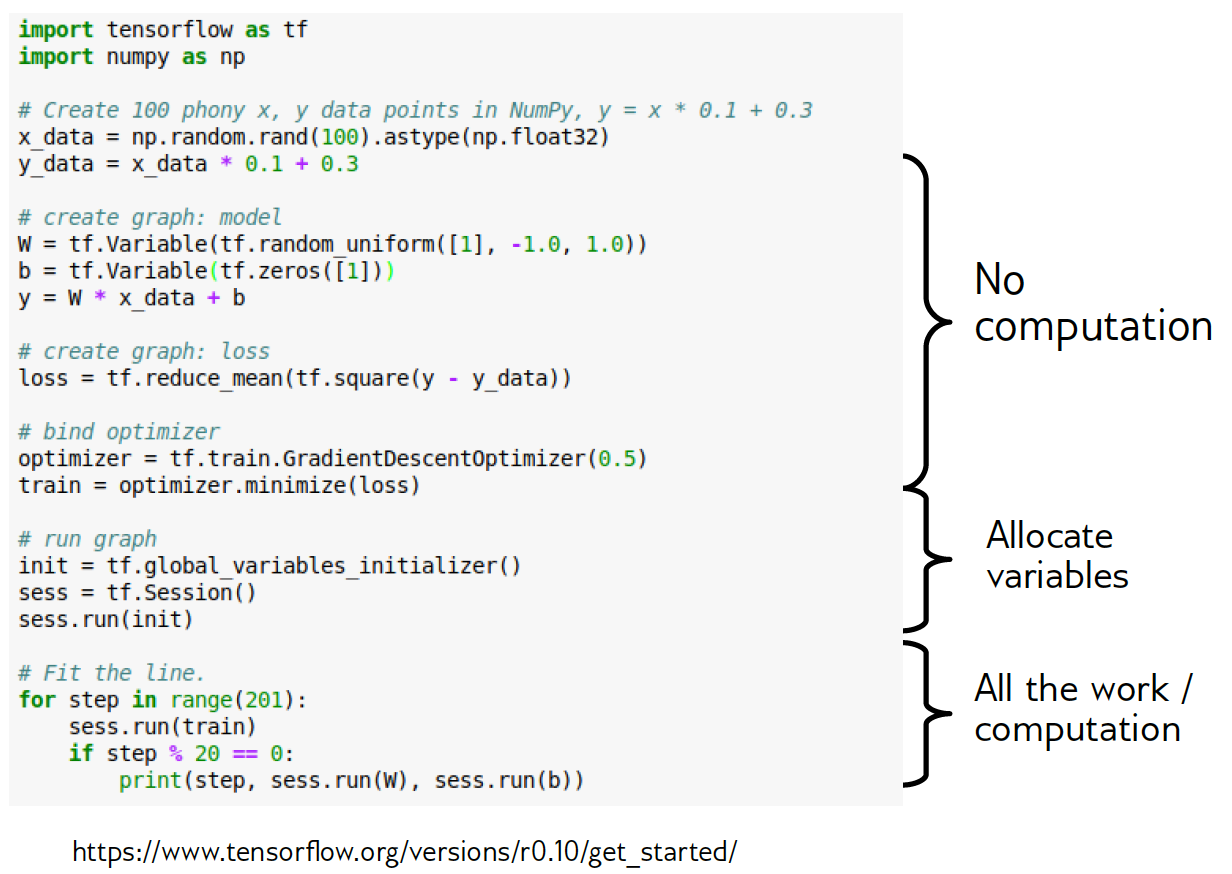
Quick Look at TensorFlow

• "Down to the metal" - don’t use for everyday tasks
• Three steps for learning:
  1. Build computation graph (using array operations and functions)
  2. Create Optimizer (gradient descent, adam, etc.) attached to graph
  3. Run actual computation

PyTorch Example

dtype = torch.float
device = torch.device("cpu")

N = 100
x = torch.randn(N, 1, device=device, dtype=dtype)
y = torch.randn(N, 1, device=device, dtype=dtype)
w = torch.randn(D_in, H, device=device, dtype=dtype)

learning_rate = 1e-6
for t in range(500):
    y_pred = x.mm(w1)
    loss = (y_pred - y).pow(2).sum().item()
    loss.backward()
    w1 -= learning_rate * w1.grad
    w1.grad.zero_()

Best Practices

• Don’t go down to the metal (i.e. write low-level code) unless you have to!
• Don’t write TensorFlow, write Keras!
• Don’t write PyTorch, write pytorch.nn or FastAI (or Skorch or ignite)

Convolutional Neural Networks

Idea #1 Behind CNNs

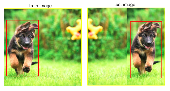
• Translation invariance: CNN can recognise an object regardless of where it is in the frame.
• … because the same filters scan every part of the image (weight sharing)

Idea #2 Behind CNNs

• Weight sharing: the principle that the same set of weights (a filter, or kernel) is used to scan every part of an image
• So, this filter will detect a specific feature (e.g. edge, curve), regardless of its position
• Each filter corresponds to a specific feature or pattern, rather than location-specific information

Why Weight Sharing?

• Reduces number of parameters; less prone to overfitting
• Comparison: for a 100x100 image with 3 channels (RGB), a fully connected layer in NN with 100 hidden units would have 3 million parameters (1001003*100);
• a convolutional layer with 10 filters of size 5x5 would have only 750 parameters (5510)

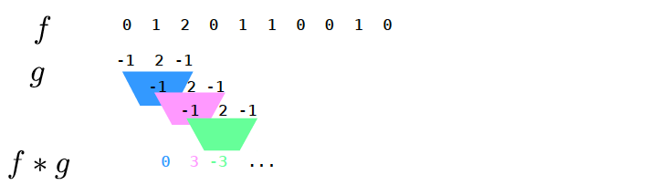
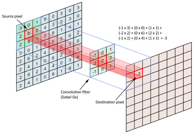
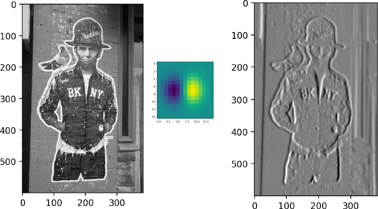
Definition of Convolution

\[(f*g)[n] = \sum\limits_{m=-\infty}^\infty f[m]g[n-m]\]

\[= \sum\limits_{m=-\infty}^\infty f[n-m]g[m]\]

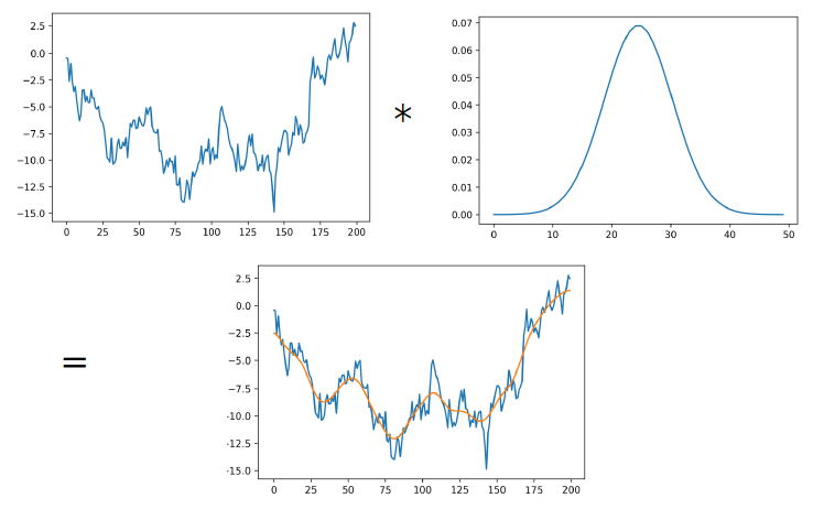
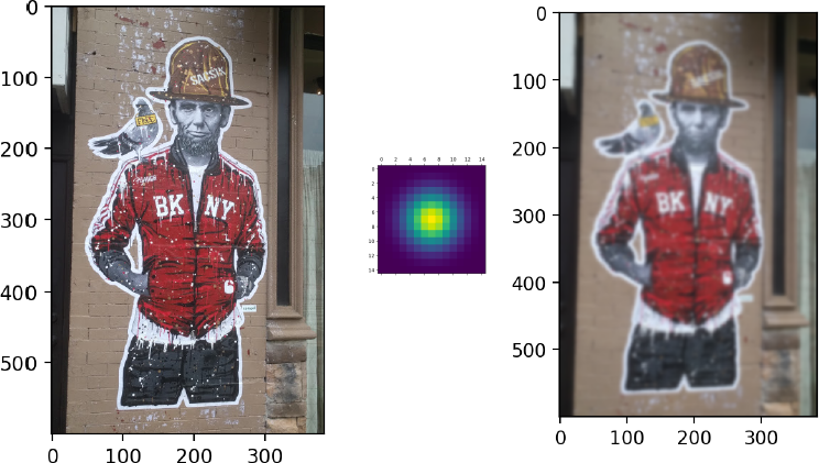
1D Example: Gaussian Smoothing

Convolutions in 2D

source: Arden Dertat

2D Convolution Animation

source: Arden Dertat

2D Smoothing

2D Gradients

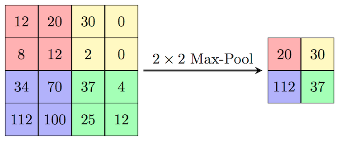
Max Pooling

• Need to remember position of maximum for back-propagation
• Again not differentiable → subgradient descent

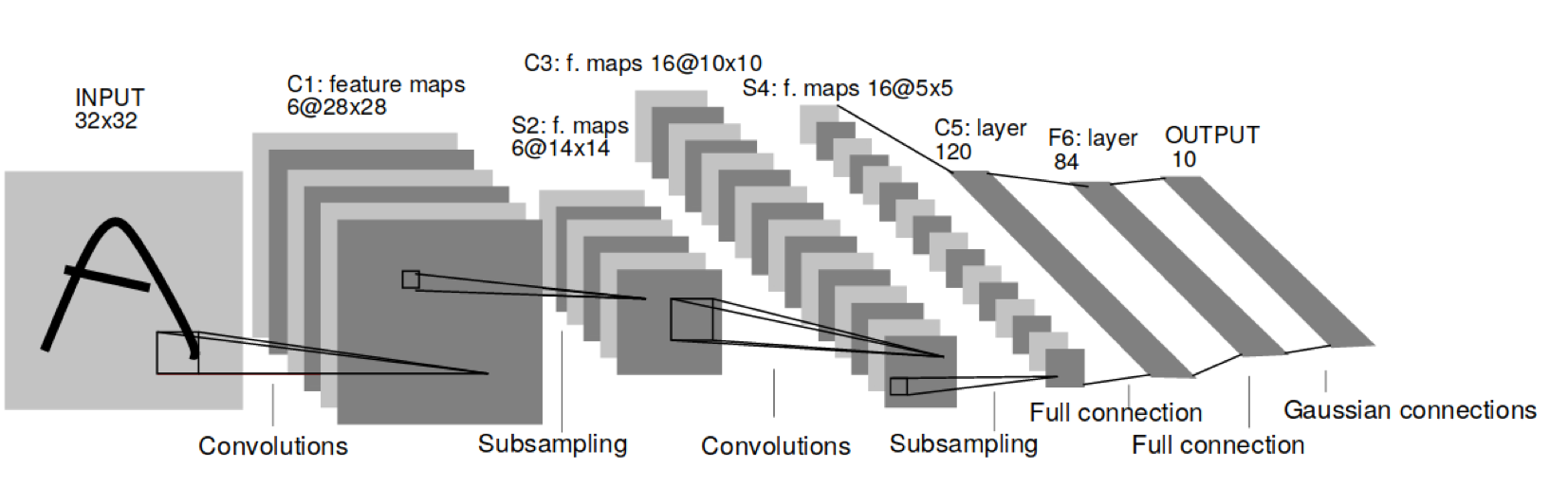
Convolutional Neural Networks

• Y. LeCun, L. Bottou, Y. Bengio, and P. Haffner: Gradient-based learning applied to document recognition

Other Architectures

Conv-nets with Keras

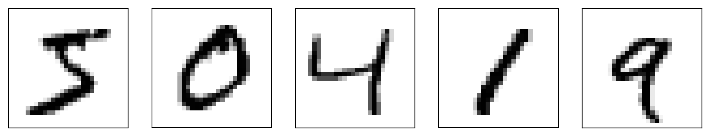
Preparing Data

batch_size = 128
num_classes = 10
epochs = 12

img_rows, img_cols = 28, 28

(x_train, y_train), (x_test, y_test) = mnist.load_data()

X_train_images = x_train.reshape(x_train.shape[0], img_rows, img_cols, 1)
X_test_images = x_test.reshape(x_test.shape[0], img_rows, img_cols, 1)
input_shape = (img_rows, img_cols, 1)

y_train = keras.utils.to_categorical(y_train, num_classes)
y_test = keras.utils.to_categorical(y_test, num_classes)

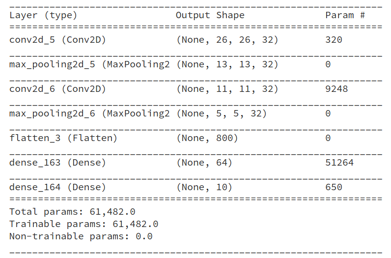
Create Tiny Network

from keras.layers import Conv2D, MaxPooling2D, Flatten

num_classes = 10
cnn = Sequential()
cnn.add(Conv2D(32, kernel_size=(3, 3),
                 activation='relu',
                 input_shape=input_shape))
cnn.add(MaxPooling2D(pool_size=(2, 2)))
cnn.add(Conv2D(32, (3, 3), activation='relu'))
cnn.add(MaxPooling2D(pool_size=(2, 2)))
cnn.add(Flatten())
cnn.add(Dense(64, activation='relu'))
cnn.add(Dense(num_classes, activation='softmax'))

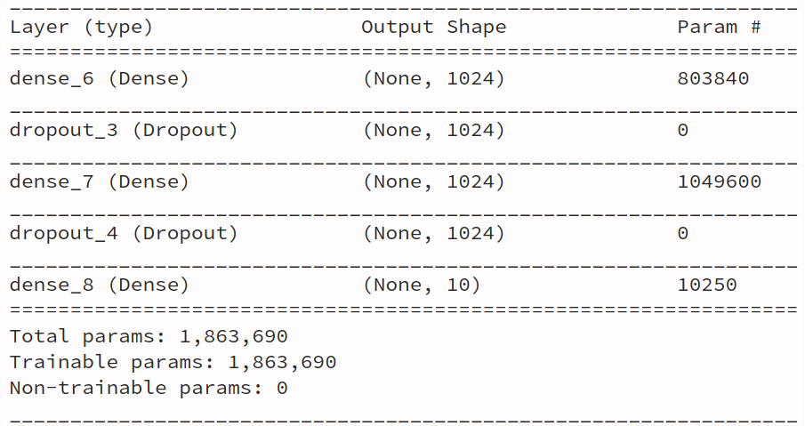
Number of Parameters

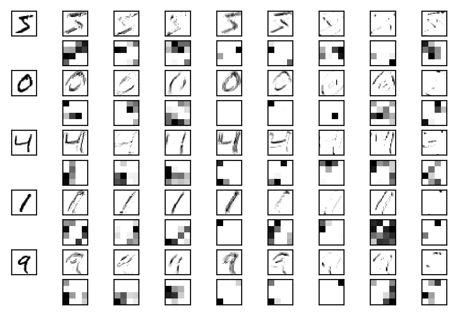
Convolutional Network for MNIST

Dense Network for MNIST

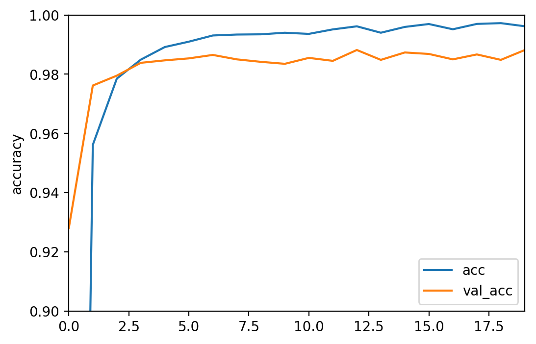
Train and Evaluate

cnn.compile(\"adam\", \"categorical_crossentropy\", metrics=['accuracy'])
history_cnn = cnn.fit(X_train_images, y_train,
                      batch_size=128, epochs=20, verbose=1, validation_split=.1)
cnn.evaluate(X_test_images, y_test)

 9952/10000 [============================>.] - ETA: 0s
 [0.089020583277629253, 0.98429999999999995]

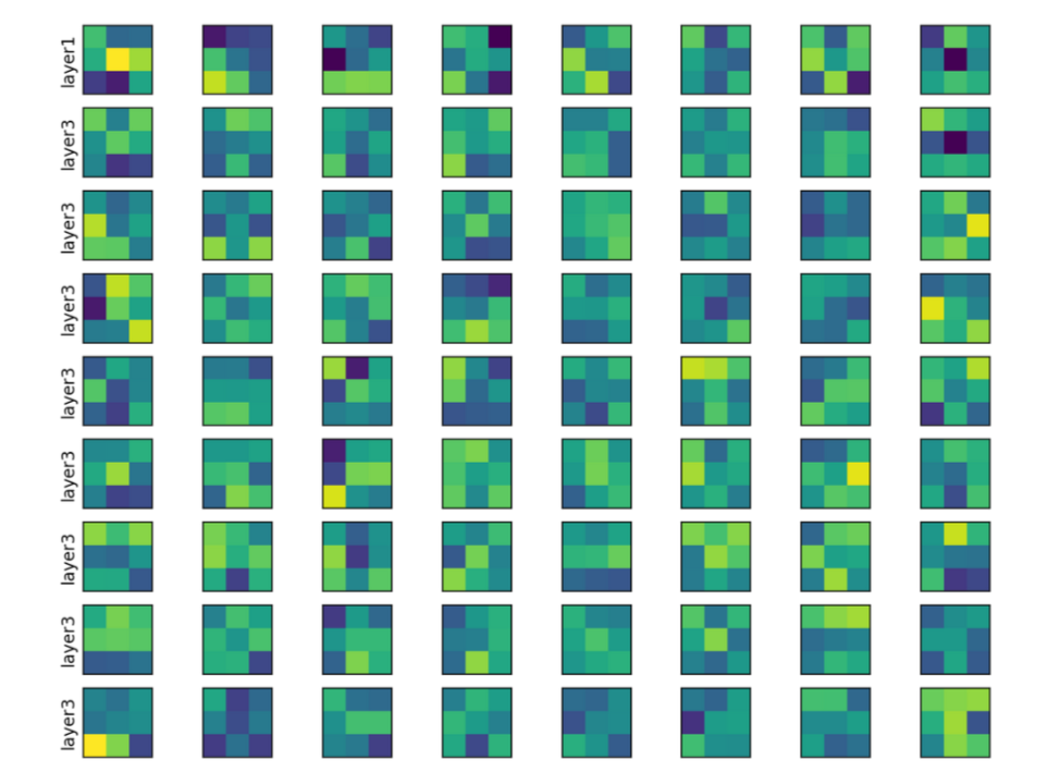
Visualise Filters

weights, biases = cnn_small.layers[0].get_weights()
weights2, biases2 = cnn_small.layers[2].get_weights()
print(weights.shape)
print(weights2.shape)

(3,3,1,8)
(3,3,8,8)

Learned Features

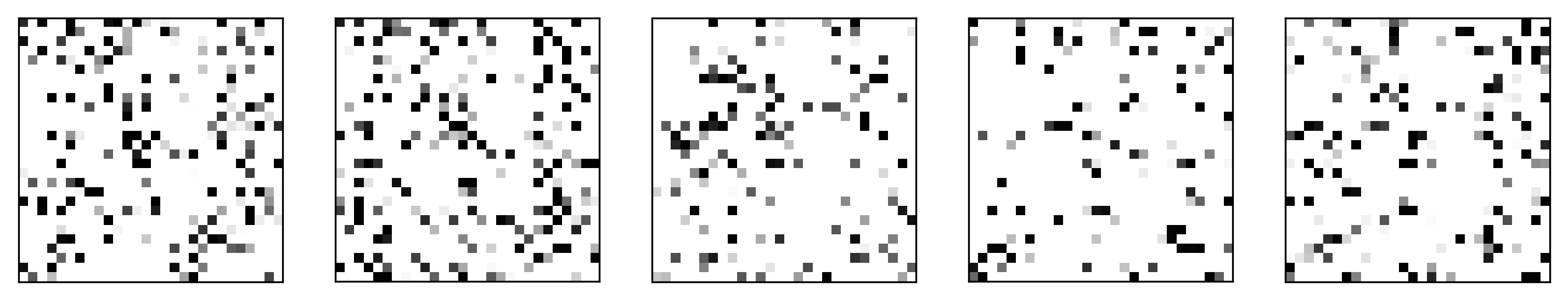
MNIST and Permuted MNIST

rng = np.random.RandomState(42)
perm = rng.permutation(784)
X_train_perm = X_train.reshape(-1, 784)[:, perm].reshape(-1, 28, 28)
X_test_perm = X_test.reshape(-1, 784)[:, perm].reshape(-1, 28, 28)

Summary

• We’ve covered the architecture and training of neural networks
• We also covered the idea and implementation of convolutional neural networks

Questions?