Tree-Based Methods

Tree, Forest, and Gradient Boosting

Huanfa Chen - huanfa.chen@ucl.ac.uk

13/12/2025

Last week

• Analysis workflow of supervised learning
• Model evaluation methods: train-test split, cross validation (and extensions)

Objectives of this week

1. Understand decision trees and tree-based ensemble methods (random forests, gradient boosting)
2. Can apply tree-based methods to real-world problems

Decision Trees

Decision Trees (DT)

• Many types of decision trees: classification and regression trees (CART), C4.5, ID3, CHAID, etc.
• Most trees (except CART) are rarely used these days, and CART is still popular.
• Focus on CART: binary trees for classification and regression
• A CART is a regression tree when the target variable Y is continous, and a classification tree when Y is categorical.
• It is not dependent on type of features (X).

Why DT?

• Non-linear, strong models for classification and regression
• Minimal preprocessing: scale and distributions matter little
• Good interpretation: small trees can be explained

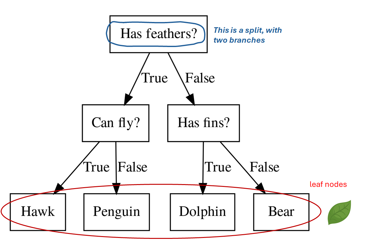
Decision Trees for Classification

• It starts with a root node
• A split with a threshold on a single X feature divides data into two parts
• Leave Nodes are the endpoints that give predictions.

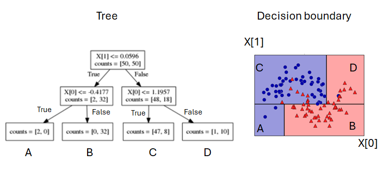
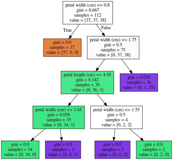
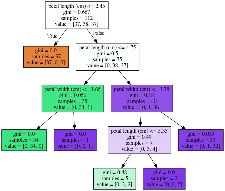
Another (synthetic) classification tree

• A dataset with two numertical features (X[0], [1]), to predict Y with two classes (RED and BLUE)
• Two visuals: tree structure, decision boundary
• The leaf node and region are one-to-one mapped.
• a node with counts=[40, 30] means this node contains 40 RED samples, 30 BLUE samples.

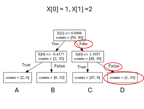
Making predictions with classification tree

• Given a new sample, start from the root node, traverse the tree according to split, until reaching a leaf node.
• Leaf node D has counts=[1, 10], so it predicts BLUE class AND probability distribution of [1/11, 10/11] over two classes.

How to build a classification tree

• A tree is built by a split from the root node, then recursively splitting child nodes.
• A key question: How to choose a split?
• Note:
  • A split is a X feature and a threshold.
  • Can’t split on Y, as Y is unknown for new datasets.
  • Can’t split on multiple X variables.
• A split is chosen to best separate Y classes, by measuring impurity reduction before & after split

To measure impurity of a node

• Gini: \(H_{\text{gini}}(X_m) = \sum_{k \in \mathcal{Y}} p_{mk}(1-p_{mk})\)
  • \(p_{mk}\) is class \(k\) proportion in node \(m\)
• The larger Gini, the more impure the node
• When Gini=0, the node is pure (all samples in one class)
• Example: a node with 10 samples in three classes [2,5,3].
• Gini = 0.2 × 0.8 + 0.5 × 0.5 + 0.3 × 0.7 = 0.66

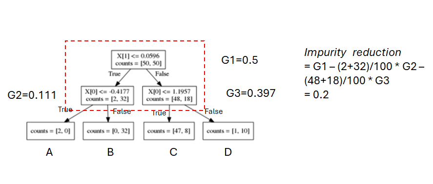
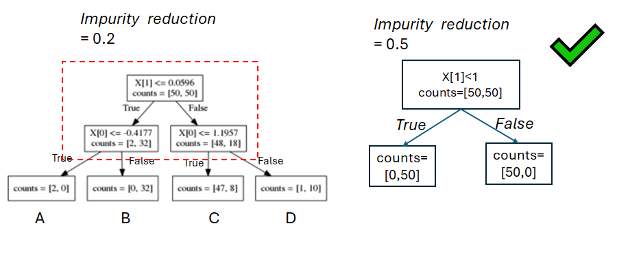
To measure impurity reduction by a split

• A good split will put similar samples together, or generate two child nodes with lower impurity
• Impurity reduction by a split = impurity(parent) - weighted impurity(children)

To choose a split

• All splits will be evaluated
• The split with the largest impurity reduction will be chosen

A regression tree

• Similar to classification tree, but a leaf node stores a range of Y values and will predict the mean of Y
• To measure impurity of a node in regresiion tree: Mean Square Error
• \(H(X_m) = \frac{1}{N_m}\sum_{i \in N_m}(y_i-\bar{y}_m)^2\)
• MSE measures the deviation of Y values from its mean, which is similar to the idea of impurity.
• If all Y values are the same, MSE=0, meaning the node is pure.

Summary of impurity measures of decision trees

• For classification:
  • Gini (by default)
  • Cross-Entropy
• For regression
  • Mean Square Error (by default)
  • Mean Absolute Error

Visualising Trees (sklearn)

from sklearn.datasets import load_breast_cancer
from sklearn.model_selection import train_test_split
from sklearn.tree import DecisionTreeClassifier

cancer = load_breast_cancer()
X_train, X_test, y_train, y_test = train_test_split(
    cancer.data, cancer.target, stratify=cancer.target, random_state=0)

tree = DecisionTreeClassifier(max_depth=2).fit(X_train, y_train)

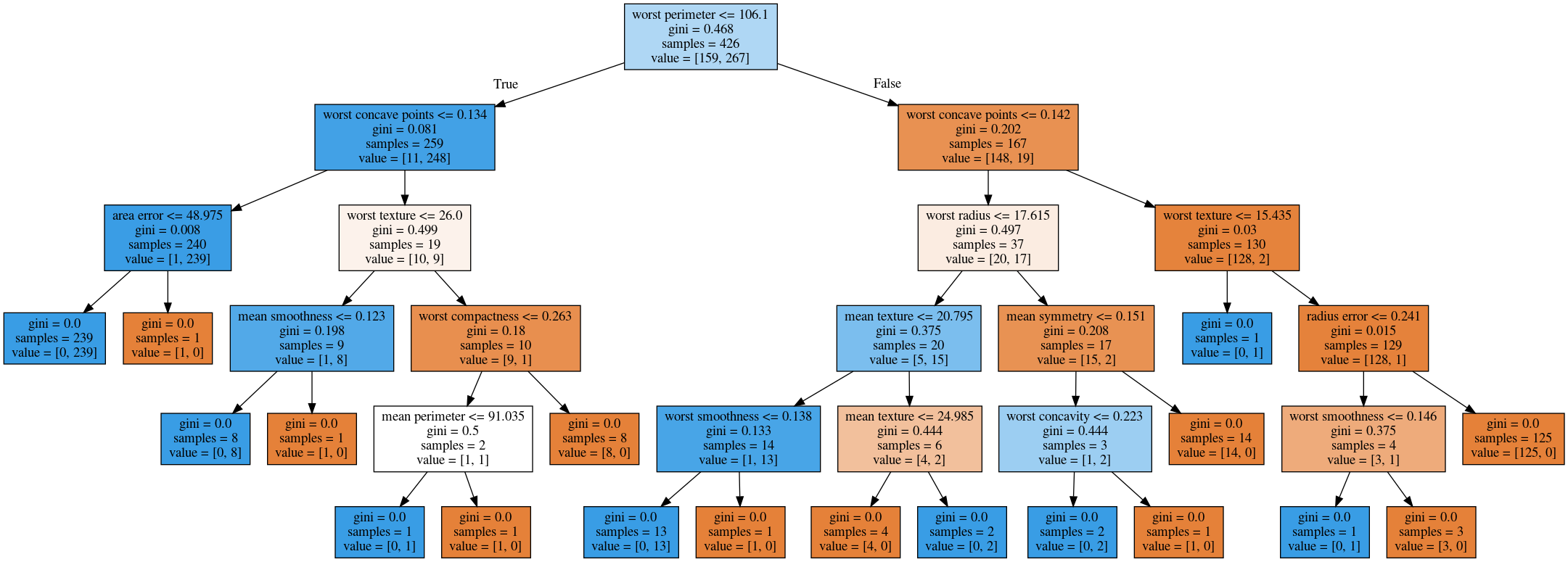
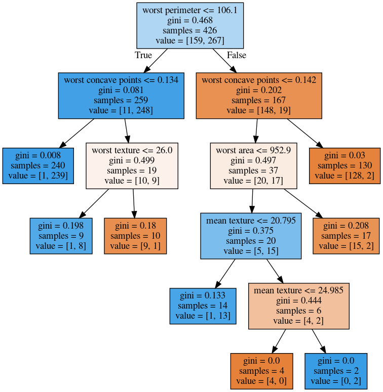
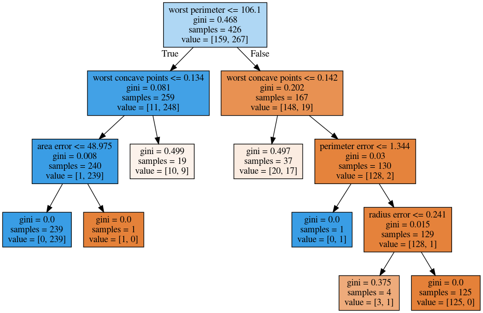
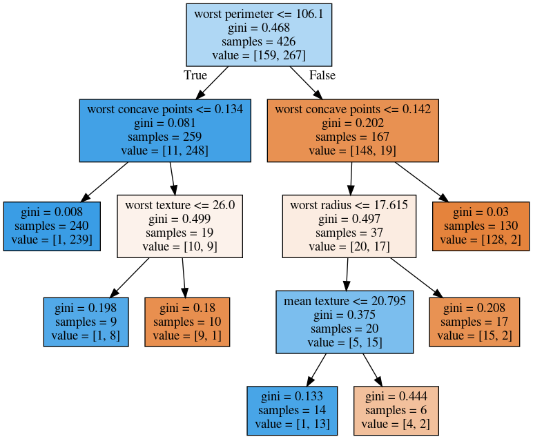
Visualising Trees (plot_tree)

from sklearn.tree import plot_tree
tree_dot = plot_tree(tree, feature_names=cancer.feature_names)

Parameter Tuning

• Pre-pruning (limit growth)
  • max_depth
  • max_leaf_nodes
  • min_samples_split
  • min_impurity_decrease
• Post-pruning (cost-complexity) after full growth

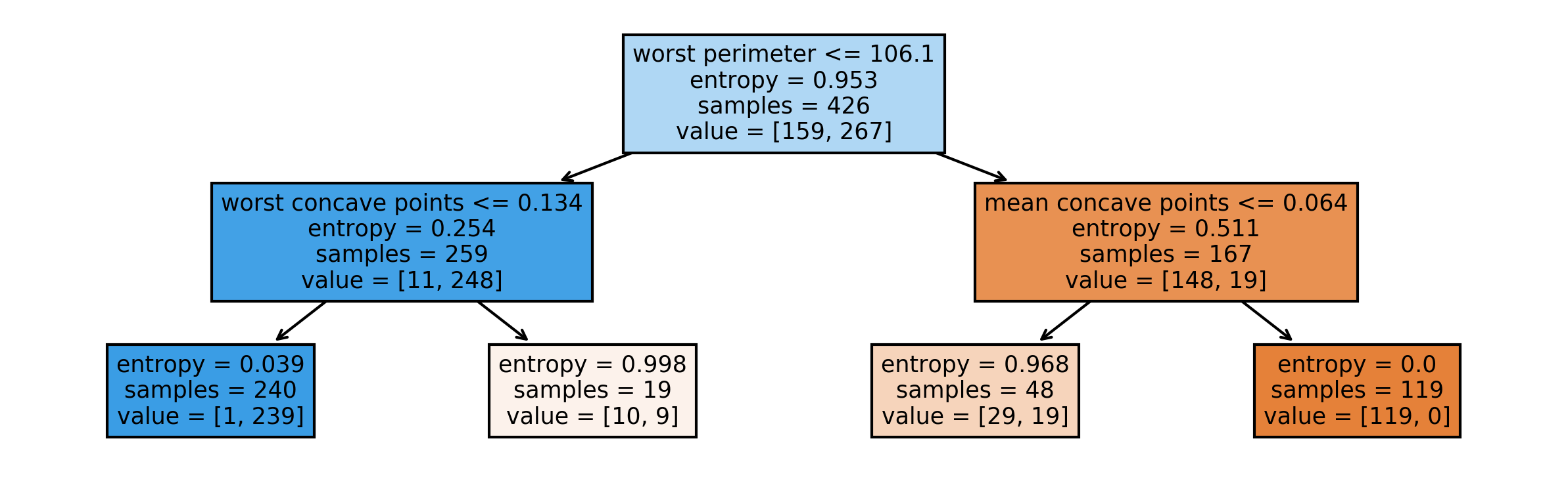
No Pruning

max_depth = 4

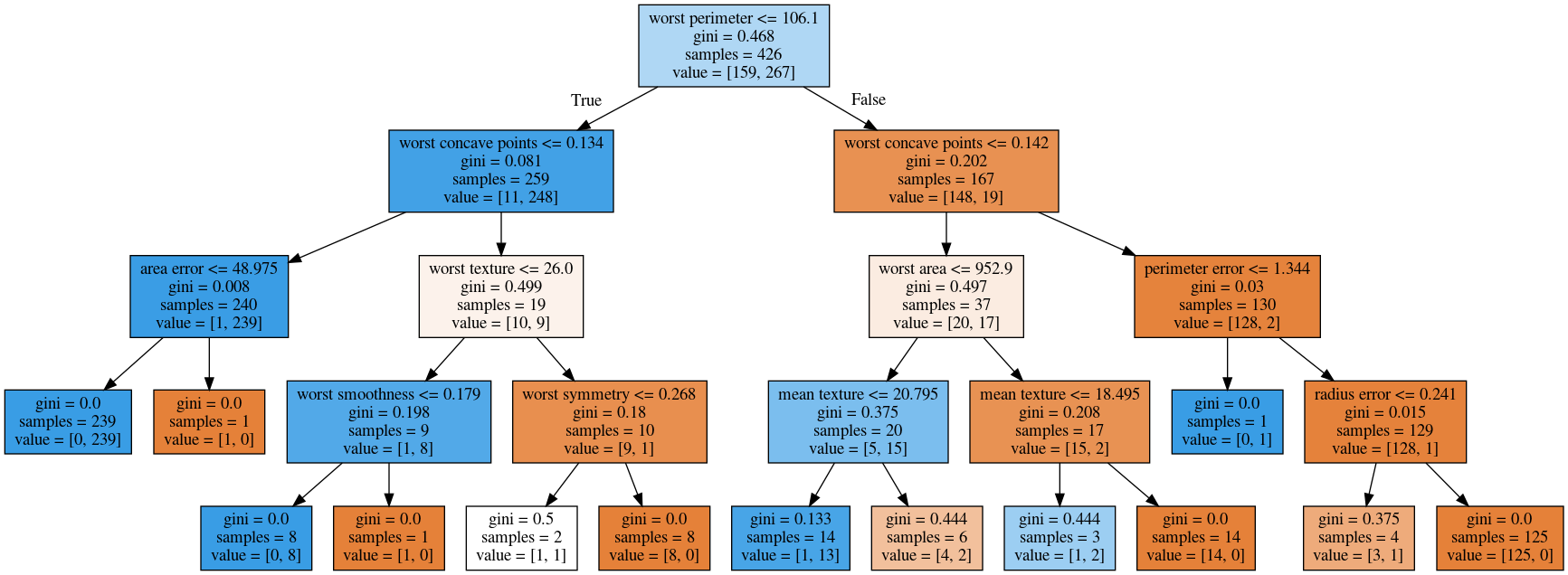
max_leaf_nodes = 8

min_samples_split = 50

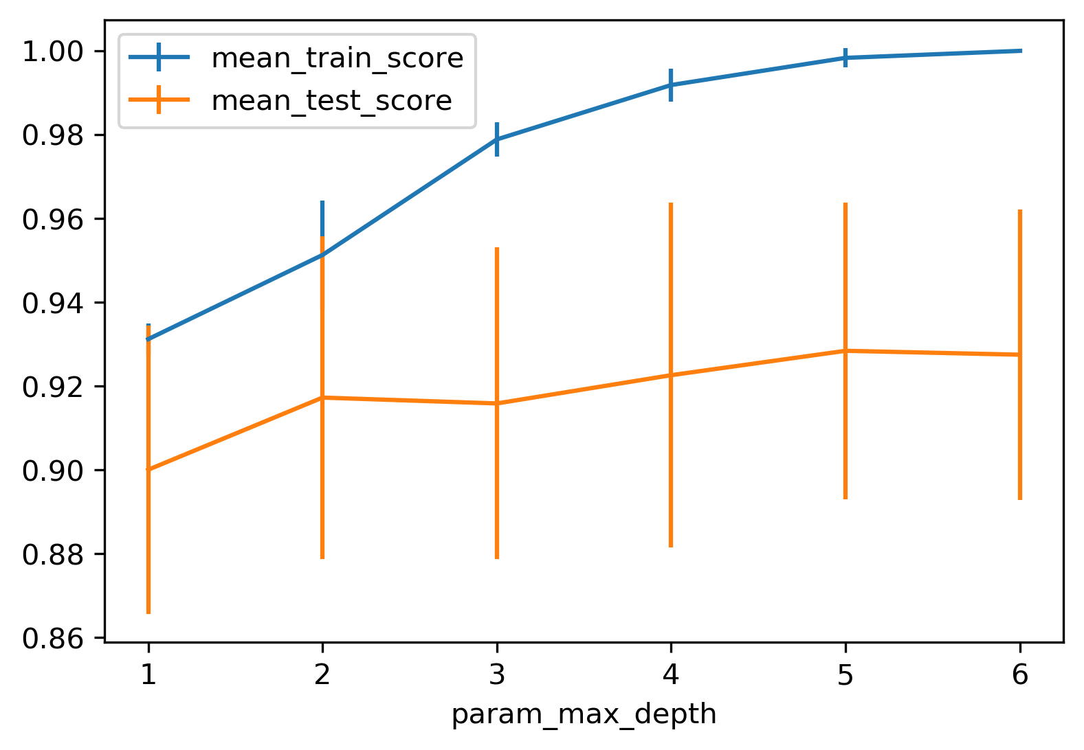
Grid Search: max_depth

from sklearn.model_selection import GridSearchCV
param_grid = {'max_depth': range(1, 7)}
grid = GridSearchCV(DecisionTreeClassifier(random_state=0),
                    param_grid=param_grid, cv=10)
grid.fit(X_train, y_train)

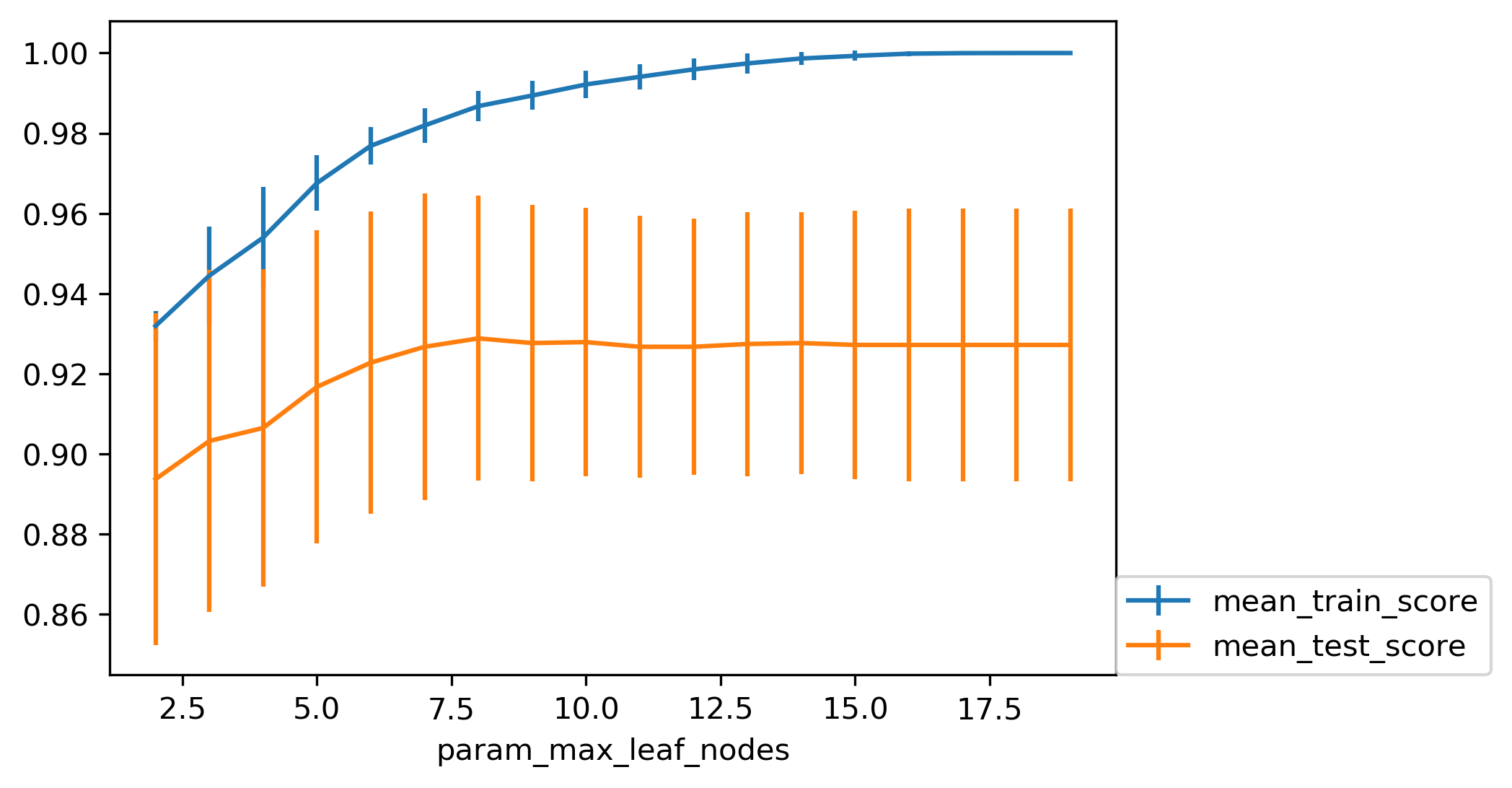
Grid Search: max_leaf_nodes

param_grid = {'max_leaf_nodes': range(2, 20)}

Cost Complexity Pruning

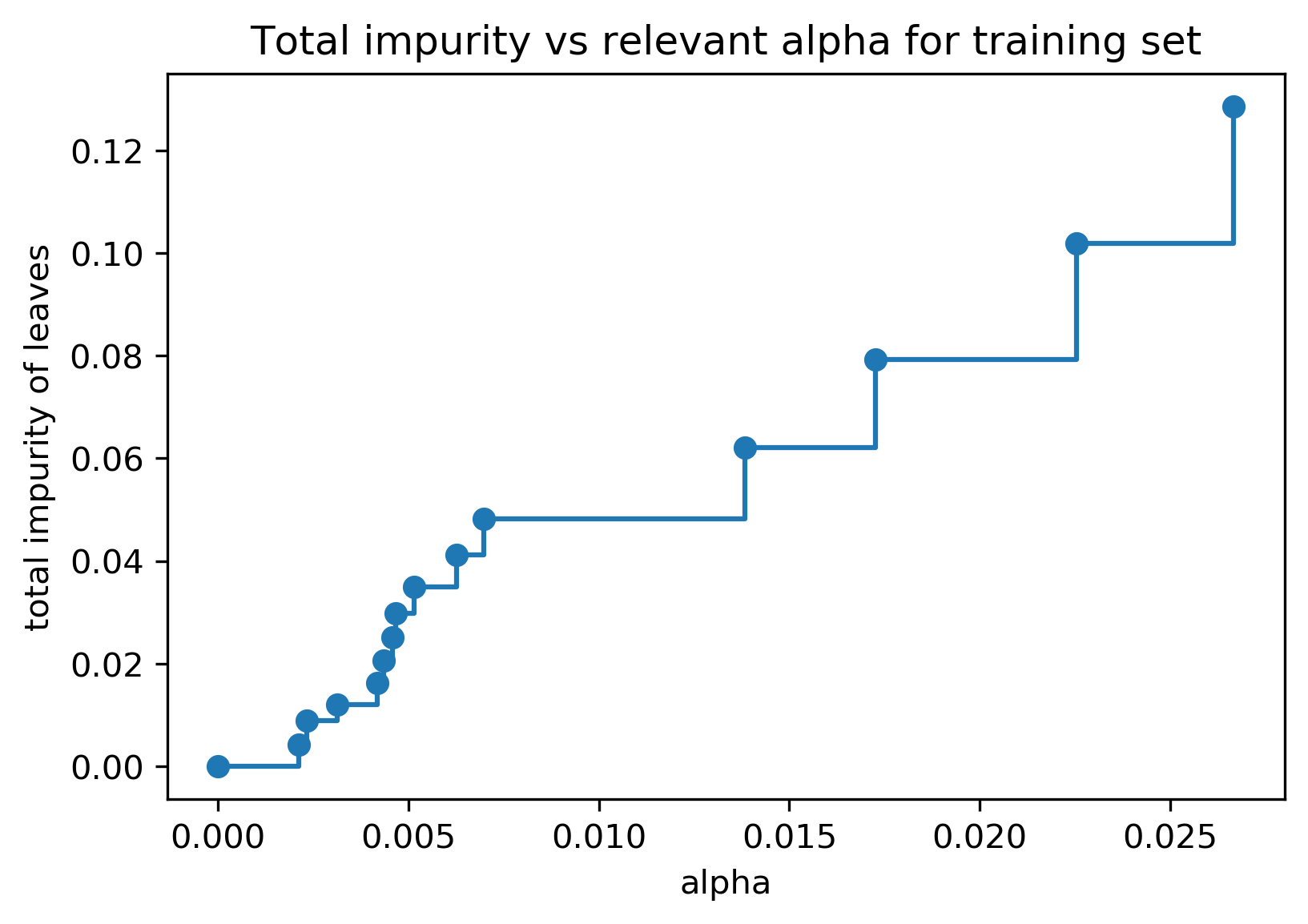
• Objective: \(R_\alpha(T) = R(T) + \alpha |T|\)
• \(R(T)\) = total leaf impurity; \(|T|\) = number of leaves; tune \(\alpha\)

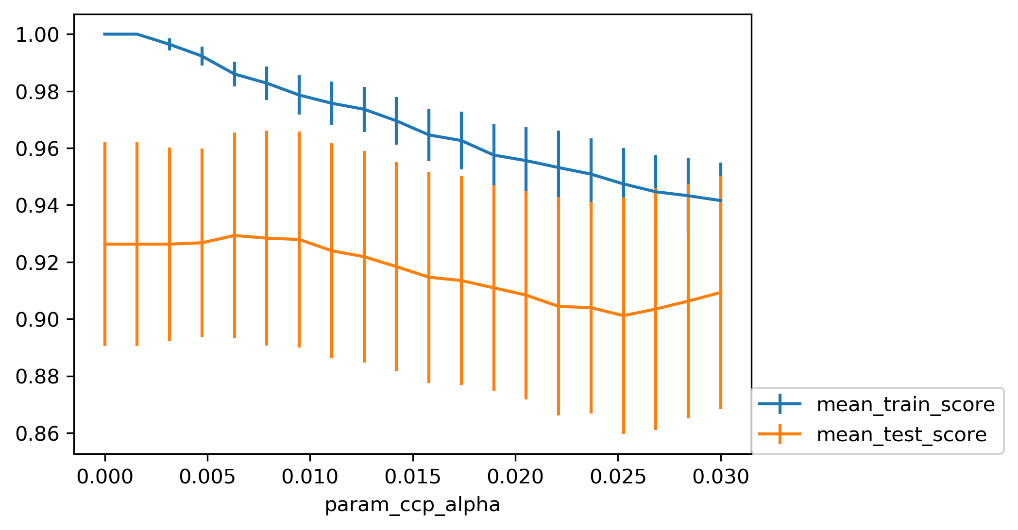
Efficient Pruning Path

clf = DecisionTreeClassifier(random_state=0)
path = clf.cost_complexity_pruning_path(X_train, y_train)
ccp_alphas, impurities = path.ccp_alphas, path.impurities

Post- vs Pre-Pruning

• Cost-complexity pruning result

  

• max_leaf_nodes search result

  

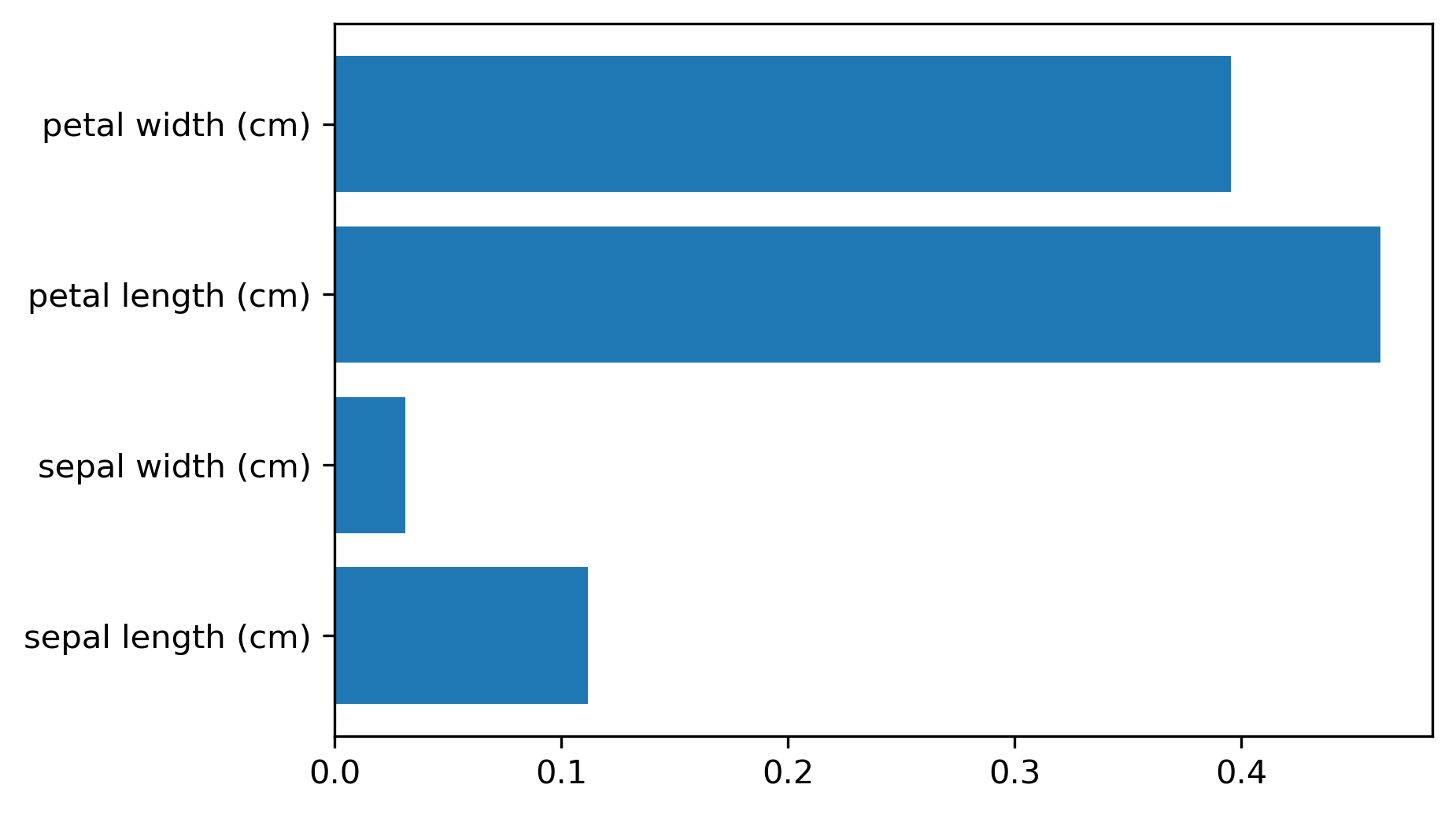
Feature Importance

from sklearn.tree import DecisionTreeClassifier
from sklearn.model_selection import train_test_split

X_train, X_test, y_train, y_test = train_test_split(
    iris.data, iris.target, stratify=iris.target, random_state=0)
tree = DecisionTreeClassifier(max_leaf_nodes=6).fit(X_train, y_train)
tree.feature_importances_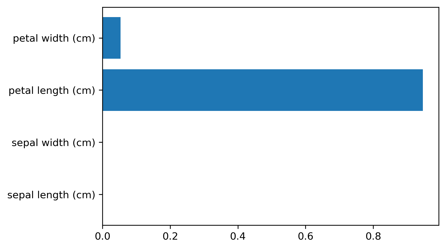

• Sum of impurity decreases per feature; magnitude only (no sign)
• Unstable with correlated features or different splits

Categorical Data

• Trees can split categories into subsets; many possible splits
• Exact search costly; efficient for binary classification + Gini
• In sklearn, one-hot encoding is needed today as sklearn can’t handle categorical features natively

Predicting Probabilities

• Leaf probability = class fraction in leaf
• e.g. for three-class leaf with samples of (AA BBB CCCCC): \(P(A)=0.2\), \(P(B)=0.3\), \(P(C)=0.5\)
• Deep, unpruned trees give overconfident (100%) probabilities
• Pruning helps but calibration may still be poor

Limitations of Trees

• Instability & overfitting: small data changes can alter splits.
• (Emsembles help)

Instability

• Small data changes can alter splits

Emsemble Methods

Poor man’s ensemble

• Combine multiple models to reduce variance / improve accuracy
• Train several models with different seeds; average predictions
• Owen Zhang (long time Kaggle 1st): build XGBoosting models with different random seeds.
• Works across model families (e.g., tree + linear + RF + NN)
• Key to success: diversity among models
• sklearn: VotingClassifier
  • soft: average the probabilities of all models and take the class with largest average probability
  • hard: let each model make a prediction and take majority vote

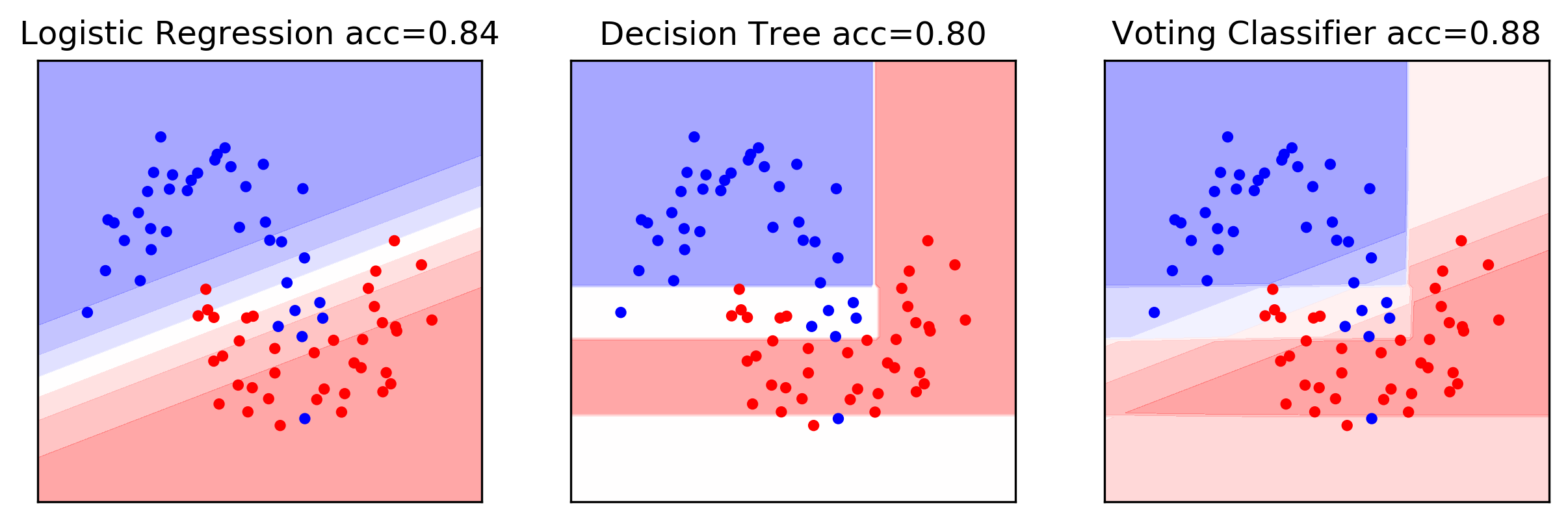
VotingClassifier Example

from sklearn.ensemble import VotingClassifier
voting = VotingClassifier(
    [('logreg', LogisticRegression(C=100)),
     ('tree', DecisionTreeClassifier(max_depth=3, random_state=0))],
    voting='soft')
voting.fit(X_train, y_train)

Tree ensemble: two types

• Bagging (Bootstrap Aggregation): random forests
• Boosting: gradient boosting machines (GBM), XGBoost, LightGBM, CatBoost, etc.

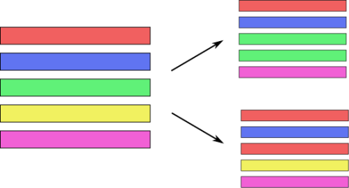
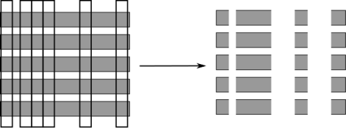
Bagging (Bootstrap Aggregation)

• Sample with replacement (same size as dataset)
• Train a model on each bootstrap sample
• Average predictions to cut variance

Bias and Variance

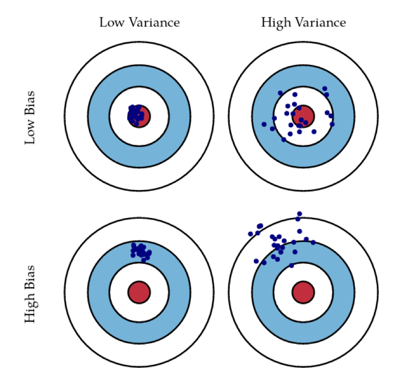
• Aim for low bias + low variance
• Averaging high-variance models can lower variance

Ensemble: Bias vs Variance

• Generalisation improves with strong base learners and low correlation
• Diversifying models (or data/features) helps more than sheer count

Random Forests

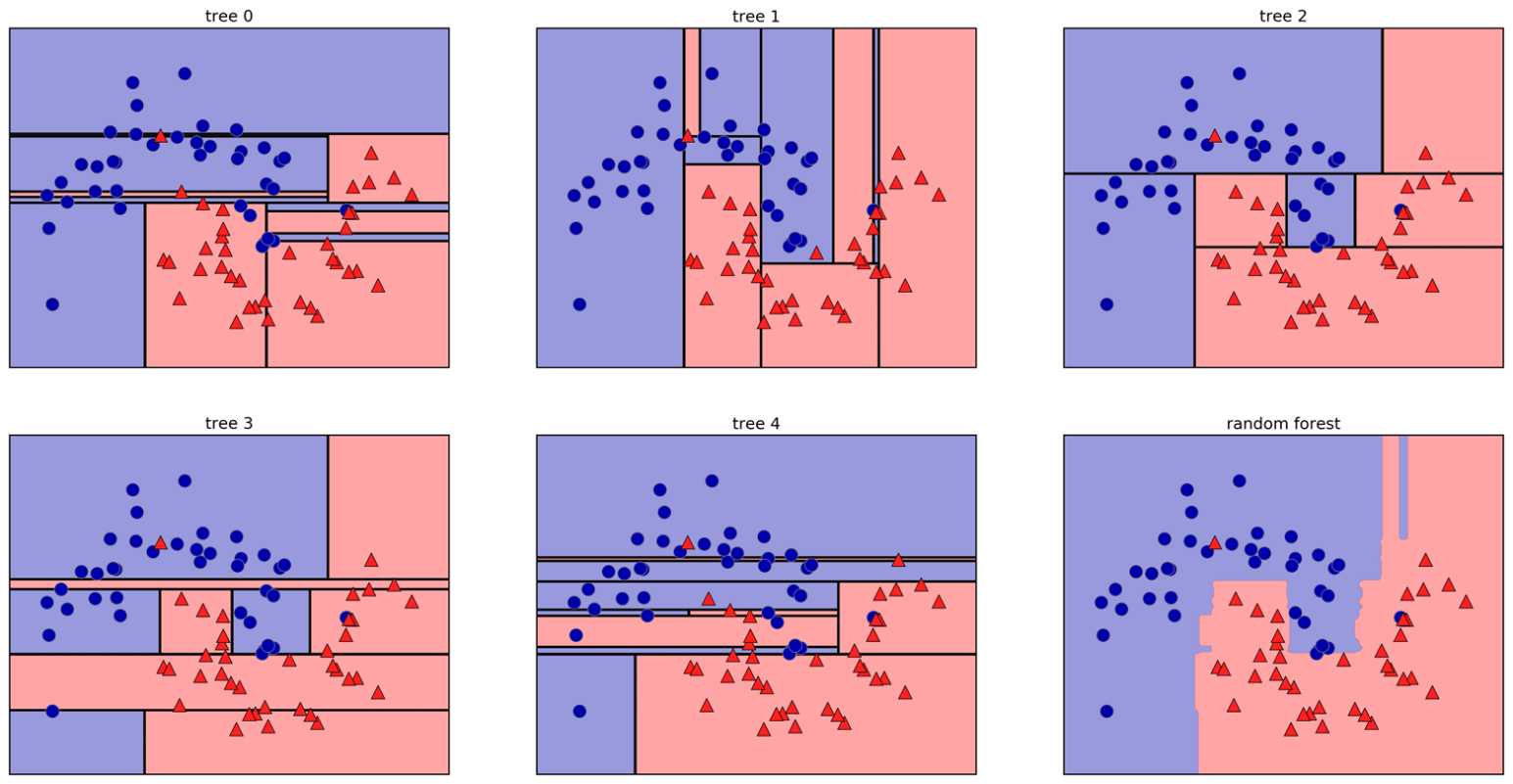
• Bagging + feature subsampling at each split

Randomise in Two Ways

• For each tree: bootstrap sample of rows
• For each split: sample features without replacement
• More trees → lower variance (diminishing returns)

Tuning Random Forests

• max_features: ~\(\sqrt{p}\) for classification, ~\(p\) for regression
• n_estimators: use 100+; more reduces variance
• Pre-pruning (max_depth, max_leaf_nodes, min_samples_split) can cut size/time

Extremely Randomized Trees

• Add randomness: draw split thresholds at random per feature
• Often no bootstrap; faster (no threshold search)
• Can yield smoother boundaries; less common than standard RF

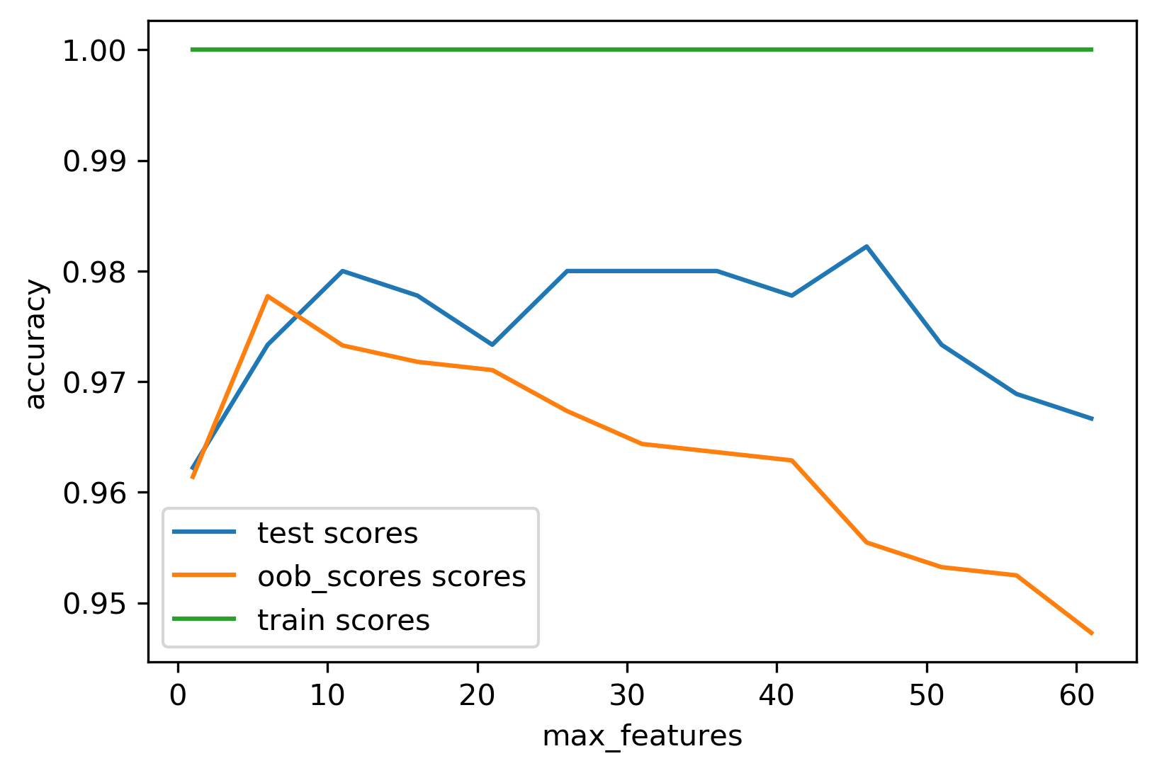
Warm-Starts

rf = RandomForestClassifier(warm_start=True)
for n in range(1, 100, 5):
    rf.n_estimators = n
    rf.fit(X_train, y_train)

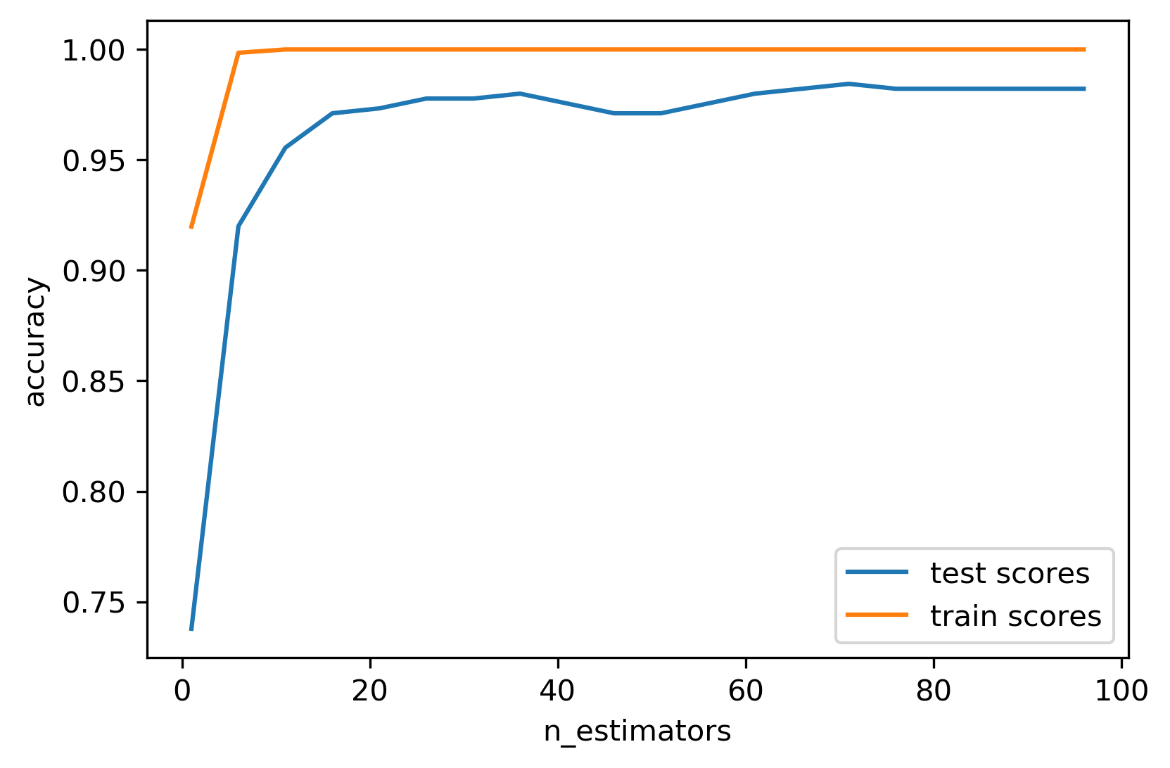
• Increase trees incrementally; stop when scores stabilise

Out-of-Bag Estimates (optional)

• Each tree trains on ~66% of data; predict remaining ~34%
• Average OOB predictions as a free validation score

rf = RandomForestClassifier(max_features=m, oob_score=True,
                            n_estimators=200, random_state=0)
rf.fit(X_train, y_train)
oob_scores.append(rf.oob_score_)

Variable Importance (RF)

rf = RandomForestClassifier().fit(X_train, y_train)
rf.feature_importances_

• More stable than single-tree importances; still magnitude-only

Trees: Takeaways

• Non-linear without heavy preprocessing
• Single small trees interpretable; forests robust baselines
• Beware extrapolation limits and instability

Gradient Boosting

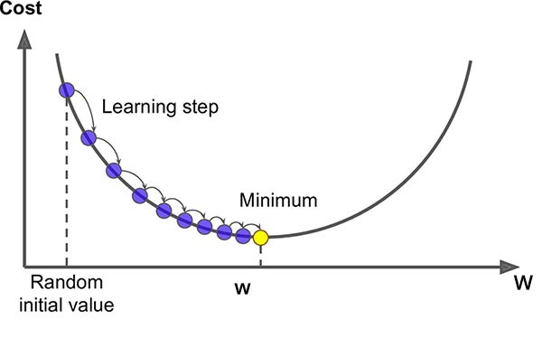
Gradient Descent

• Optimise \(\arg\min_w F(w)\) by stepping along \(-\nabla F(w)\)
• Update: \(w_{i+1} = w_i - \eta_i \nabla F(w_i)\)
• Converges to a local minimum (global for convex losses)

Stochastic Gradient Descent

• Logistic regression objective: log-loss + regularizer
• SGD uses one (or a mini-batch of) example(s) per step to approximate the gradient
• Faster on large data; noisier updates

from sklearn.linear_model import SGDClassifier
sgd = SGDClassifier().fit(X_train, y_train)

Gradient Boosting Idea

• Train a small tree to predict \(y\)
• Train next tree on residuals of previous model (or on points poorly predicted)
• Repeat; sum scaled predictions: \(f(x)=\sum \gamma g_k(x)\) with learning rate \(\gamma\)

Gradient Boosting Algorithm

\[ \begin{aligned} f_{1}(x) &\approx y \\ f_{2}(x) &\approx y - \gamma f_{1}(x) \\ f_{3}(x) &\approx y - \gamma f_{1}(x) - \gamma f_{2}(x) \end{aligned} \]

• Each new tree fixes remaining error
• Small \(\gamma\) (e.g., 0.1) for smoother learning

Gradient Boosting as Gradient Descent

• Linear regression minimizes \(\sum (y - w^T x - b)^2\)
• Gradient descent updates weights

• Gradient boosting minimises same loss over predictions \(\hat{y}\)
• Update \(\hat{y}\) by adding trees along negative gradient

Regression Example

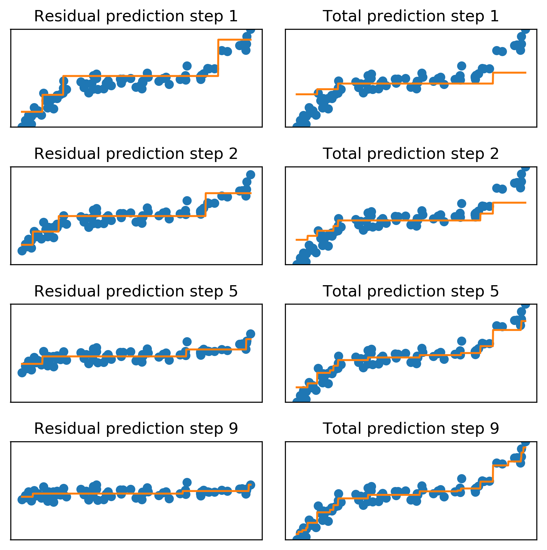
• Shallow trees fit residuals sequentially until residuals shrink

Classification Example

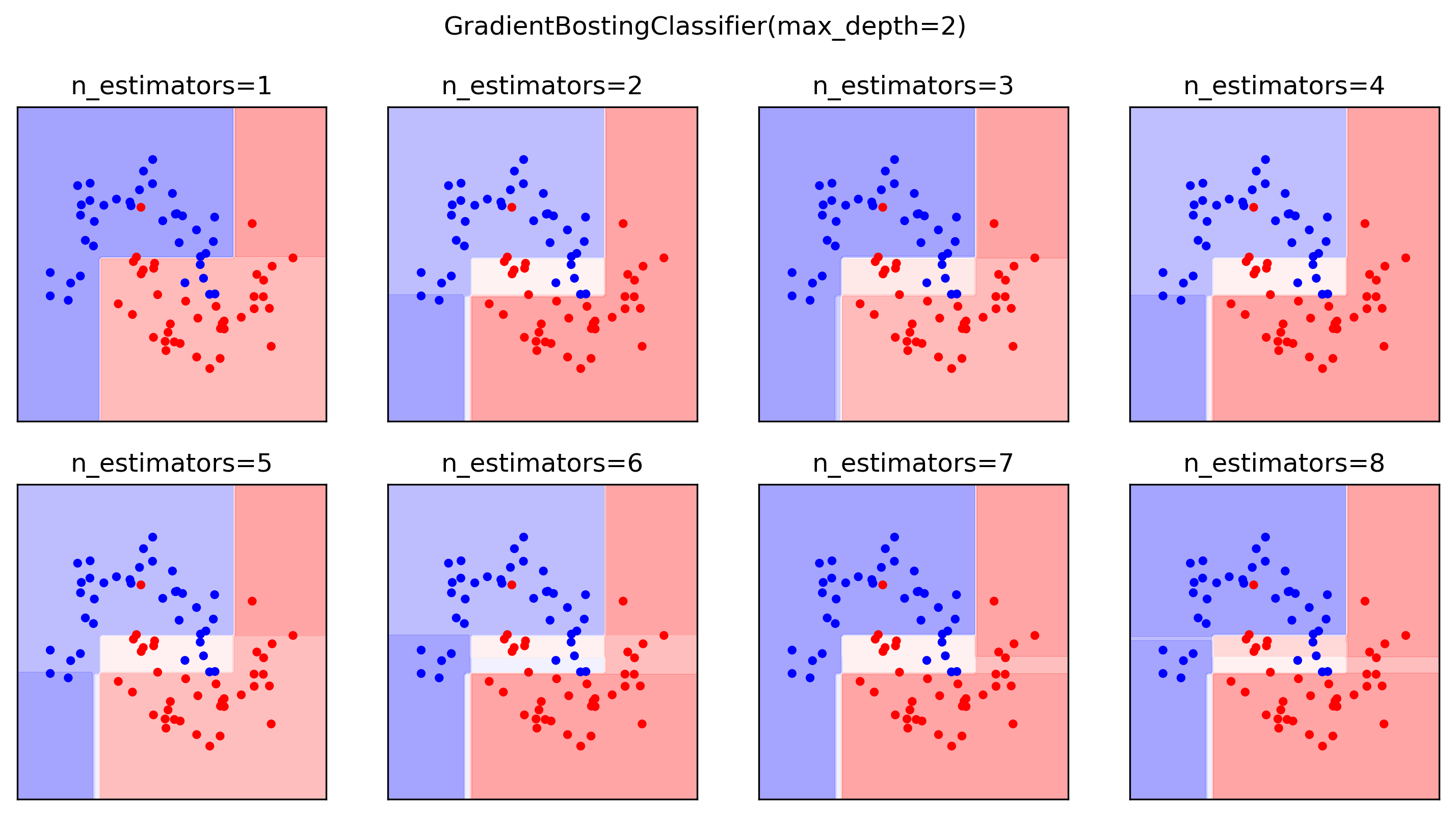
• Probability surfaces become sharper as trees accumulate
• Multiclass: one regression tree per class per step

Early Stopping

• More trees can overfit
• Stop when validation metric stops improving
• Either fix \(n_{\text{estimators}}\) and tune \(\gamma\), or fix \(\gamma\) and stop early

Tuning Gradient Boosting

• Use shallow trees (strong pruning via max_depth)
• Tune learning rate, n_estimators, subsampling of rows/columns
• Optional regularisation (min_samples_split, min_impurity_decrease)

Ensuring uncorrelated trees: Aggressive Subsampling

• Row and column subsampling reduce correlation and overfitting
• Common in XGBoost/LightGBM

XGBoost

from xgboost import XGBClassifier
xgb = XGBClassifier().fit(X_train, y_train)

• Fast, supports missing values, GPU/cluster training
• L1/L2 on leaves; fast approximate splits; sparse data friendly

LightGBM

from lightgbm.sklearn import LGBMClassifier
lgbm = LGBMClassifier().fit(X_train, y_train)

• Native categorical handling; missing values; GPU/cluster support

CatBoost

from catboost.sklearn import CatBoostClassifier
catb = CatBoostClassifier().fit(X_train, y_train)

• Strong on categorical data; symmetric trees; target-encoding tricks; GPU

Advantages of Gradient Boosting

• Often more accurate than random forests with tuning
• Small models; fast prediction
• Hist/XGB/LightGBM implementations are very fast

Summary: when to use a tree or tree ensemble

• For tabular data
• Can model non-linear relationships and require minimal preprocessing
• Single small tree for interpretability, but a single tree often underfits and doesn’t generalise well
• Random forests are very robust and good benchmark
• Gradient boosting generate best accuracy when tuned

Questions