Practical 3: Supervised learning workflow

This week will introduce the supervised learning framework and key metrics for evaluating supervised learning models using the London Fire Brigade dataset.

Learning Outcomes

You have familiarised yourself with the key concepts of supervised machine learning workflow, including train-test split, cross validation, and hyperparameter tuning.
You are able to explain the differences between different workflows, including their pros and cons.

Starting the Practical

The process for every week will be the same: download the notebook to your DSSS folder (or wherever you keep your course materials), switch over to JupyterLab (which will be running in Podman/Docker) and get to work.

If you want to save the completed notebook to your Github repo, you can add, commit, and push the notebook in Git after you download it. When you’re done for the day, save your changes to the file (this is very important!), then add, commit, and push your work to save the completed notebook.

Note

Suggestions for a Better Learning Experience:

Set your operating system and software language to English: this will make it easier to follow tutorials, search for solutions online, and understand error messages.
Save all files to a cloud storage service: use platforms like Google Drive, OneDrive, Dropbox, or Git to ensure your work is backed up and can be restored easily when the laptop gets stolen or broken.
Avoid whitespace in file names and column names in datasets

Revisiting London Fire Brigade Dataset

This week, we will continue using the London Fire Brigade (LFB) dataset for supervised learning tasks. For the context of LFB data and the two learning tasks, please refer to Week 2 practical notebook. Briefly, we formulated two supervised learning tasks using the LFB dataset and have got some initial results:

Regression: predicting daily LFB callouts in Greater London, using weather and temporal features.
Classification: predicting whether a fire incident is a false alarm given the location available at the time of the callout, which includes time of day, day of week, building type (dwelling or commercial).

Predicting daily LFB callouts

Remember in predicting daily LFB callouts, we used a random forest model and a train-test split:

# import data from https://raw.githubusercontent.com/huanfachen/DSSS_2025/refs/heads/main/data/LFB_2023_daily_data.csv
import pandas as pd
df_lfb_daily = pd.read_csv("https://raw.githubusercontent.com/huanfachen/DSSS_2025/refs/heads/main/data/LFB_2023_daily_data.csv")

# using Random Forest to predict IncidentCount using weather, weekday, weekend, and bank holiday info
from sklearn.ensemble import RandomForestRegressor
from sklearn.model_selection import train_test_split, GridSearchCV
from sklearn.metrics import mean_squared_error, r2_score

# prepare data for modeling
feature_cols = ['TX', 'TN', 'TG', 'SS', 'SD','RR','QQ', 'PP','HU','CC', 'IsWeekend', 'IsBankHoliday', 'weekday']
X = df_lfb_daily[feature_cols]
y = df_lfb_daily['IncidentCount']

# one-hot encode the 'weekday' column
X = pd.get_dummies(X, columns=['weekday'], drop_first=True)

# split data into training and testing sets
X_train, X_test, y_train, y_test = train_test_split(X, y, test_size=0.2, random_state=42)

# train Random Forest model
model = RandomForestRegressor(random_state=42)
model.fit(X_train, y_train)

# evaluate model performance on training and testing sets
y_pred_train = model.predict(X_train)
y_pred_test = model.predict(X_test)

# compute R-squared on training and testing data
r2_train = r2_score(y_train, y_pred_train)
r2_test = r2_score(y_test, y_pred_test)

print(f'Train R-squared: {r2_train:.3f}')
print(f'Test R-squared: {r2_test:.3f}')

Train R-squared: 0.918
Test R-squared: 0.180

It is obvious that the model trained is overfitting the training data, as the \(R^2\) on the training and testing data is around 0.92 and only 0.18, respectively. Therefore, this model is not useful in practice, as it doesn’t generalise well to unseen data.

To mitigate this issue, we can use cross-validation to tune the hyperparameters of the random forest model to reduce overfitting. The hyperparameters to tune include the following (see link for details):

max_depth: maximum depth of the tree (default at None, meaning nodes are expanded until all leaves are pure or until all leaves contain less tha nmin_samples_split samples)
min_samples_leaf: minimum number of samples required to be at a leaf node (default at 1)
max_features: number of features to consider when looking for the best split (default to 1.0, meaning all features are considered)

We haven’t introduced random forest algorithm yet, which is the content of Week 4. For now, please assume that these hyperparameters can control the complexity of the random forest model, and tuning them can help reduce overfitting.

Cross-validation and grid search

Cross-validation and grid search are techniques to tune hyperparameters and evaluate model performance more robustly.

In k-fold cross-validation, the training data is split into k folds, and the model is trained on k-1 folds and validated on the remaining fold. This process is repeated k times, with each fold used as the validation set once. The average performance across all folds is used to evaluate the model.

In grid search, a set of hyperparameter values is defined, and the model is trained and evaluated for each combination of hyperparameters using cross-validation. The combination that yields the best average performance across all folds is selected as the optimal hyperparameter set.

Estimating the computing time of cross-validation with grid search is key to planning the experiment, especially with large datasets or complex models. The total number of models to train is equal to the number of hyperparameter combinations multiplied by the number of folds in cross-validation. For example, if we have 3 hyperparameters with 4, 3, and 3 possible values, respectively, and we use 5-fold cross-validation, the total number of models to train is \(4 \times 3 \times 3 \times 5 = 180\).

The time for training a single model is estimated as below:

import time
model = RandomForestRegressor(random_state=42)
start_time = time.time()
model.fit(X_train, y_train)
end_time = time.time()
training_time = end_time - start_time
print(f'Training time: {training_time:.3f} seconds')

Training time: 0.189 seconds

This training took around 0.28 seconds on my desktop, so the total time for cross-validation with grid search would be approximately \(180 \times 0.28 = 50.4\) seconds, less than 1 minute.

We will start with defining the hyperparameters to tune and their possible values. The first value of max_depth and min_samples_leaf is their default value in RandomForestRegressor, respectively. See link.

# 5-fold CV to tune RandomForestRegressor

# the code below is a duplicate of the above code for data preparation

# import pandas as pd
# from sklearn.model_selection import train_test_split, GridSearchCV
# from sklearn.ensemble import RandomForestRegressor
# from sklearn.metrics import r2_score

# df_lfb_daily = pd.read_csv("https://raw.githubusercontent.com/huanfachen/DSSS_2025/refs/heads/main/data/LFB_2023_daily_data.csv")

# feature_cols = ['TX', 'TN', 'TG', 'SS', 'SD','RR','QQ', 'PP','HU','CC', 'IsWeekend', 'IsBankHoliday', 'weekday']
# X = df_lfb_daily[feature_cols]
# y = df_lfb_daily['IncidentCount']
# X = pd.get_dummies(X, columns=['weekday'], drop_first=True)

# # split data
# X_train, X_test, y_train, y_test = train_test_split(X, y, test_size=0.2, random_state=42)

param_grid = {
  'max_depth': [None, 5, 10, 20],
  'min_samples_leaf': [1, 2, 4],
  'max_features': ['sqrt', 'log2', 0.5]
}

We will then use GridSearchCV function from sklearn.model_selection to perform grid search with 5-fold cross-validation to find the optimal hyperparameters. This function is very handy, as it automatically handles the cross-validation and hyperparameter tuning. Moreover, we will fit the grid search object on the training data just like how we fit a model. The power of interface design.

After fitting, we can access the best hyperparameters and the best cross-validated \(R^2\) using the best_params_ and best_score_ attributes, respectively. Then, we will retrain the final model using the optimal hyperparameters on the entire training data and evaluate its performance on both the training and testing data.

start_time = time.time()
grid = GridSearchCV(
  estimator=RandomForestRegressor(random_state=42),
  param_grid=param_grid,
  cv=5,
  scoring='r2',
  n_jobs=-1, # n_jobs=-1 use all available cores
  return_train_score=True
)

grid.fit(X_train, y_train)

# print best hyperparameters and best CV R-squared
print("Best hyperparameters:", grid.best_params_)
print(f"Best CV R-squared: {grid.best_score_:.3f}")

end_time = time.time()
training_time = end_time - start_time
print(f'CV training time: {training_time:.3f} seconds')

# retrain with optimal hyperparameters
best_params = grid.best_params_
best_model = RandomForestRegressor(random_state=42, **best_params)
best_model.fit(X_train, y_train)

# r2 on training and testing data
train_r2 = r2_score(y_train, best_model.predict(X_train))
print(f"Train R-squared: {train_r2:.3f}")
test_r2 = r2_score(y_test, best_model.predict(X_test))
print(f"Test R-squared: {test_r2:.3f}")

Best hyperparameters: {'max_depth': 10, 'max_features': 'sqrt', 'min_samples_leaf': 1}
Best CV R-squared: 0.368
CV training time: 10.760 seconds
Train R-squared: 0.860
Test R-squared: 0.200

The GridSearchCV took around 3.66 seconds on my desktop, which is much faster than the estimated time. This is because the n_jobs=-1 argument allows parallel processing and using all processors, which speeds up the computation significantly.

The best hyperparameters found are as follows: - max_depth: 10 - max_features: ‘sqrt’ - min_samples_leaf: 1

And the \(R^2\) on the training, testing, and cross-validated data are as follows:

Training data: 0.860
Testing data: 0.200
CV: 0.368

The \(R^2\) on the training data has decreased from 0.92 to 0.86, while the \(R^2\) on the testing data has increased from 0.18 to 0.20, indicating that the overfitting issue has been mitigated to some extent. Note that the cross-validated \(R^2\) is higher than the testing \(R^2\), which indicates that the model is overfitting during cross validation and the best way to evaluate the model is using the unseen testing data.

A real prediction task

Now that we have a trained model that can predict the daily LFB callouts. However, this model is not really trained on the past data, as we use a random train-test split and a random CV. This might overestimate the model performance, as the model might have seen future data during training.

In a real prediction task, we should use a temporal train-test split, where the training data is from the past and the testing data is from the future. In the next part, we will use the first 80% data (sorted by date) for training and the remaining data for testing.

Please note that the analysis below doesn’t generate high predictive accuracy. Rather, this analysis serves as an example of how to implement temporal train-test split and temporal cross-validation in practice.

Temporal train-test split

import pandas as pd
from sklearn.ensemble import RandomForestRegressor
from sklearn.metrics import r2_score

# load and sort by date to respect time order
df_lfb_daily = pd.read_csv("https://raw.githubusercontent.com/huanfachen/DSSS_2025/refs/heads/main/data/LFB_2023_daily_data.csv")
df_lfb_daily['DateOfCall'] = pd.to_datetime(df_lfb_daily['DateOfCall'])

# sort by date
df_lfb_daily = df_lfb_daily.sort_values('DateOfCall')

feature_cols = ['TX', 'TN', 'TG', 'SS', 'SD','RR','QQ', 'PP','HU','CC', 'IsWeekend', 'IsBankHoliday', 'weekday']
X = df_lfb_daily[feature_cols]
y = df_lfb_daily['IncidentCount']
X = pd.get_dummies(X, columns=['weekday'], drop_first=True)

# temporal split: first 80% dates for training, remaining 20% for testing
split_idx = int(len(X) * 0.8)
X_train, X_test = X.iloc[:split_idx], X.iloc[split_idx:]
y_train, y_test = y.iloc[:split_idx], y.iloc[split_idx:]

rf = RandomForestRegressor(random_state=42)
rf.fit(X_train, y_train)

train_r2 = r2_score(y_train, rf.predict(X_train))
test_r2 = r2_score(y_test, rf.predict(X_test))

print(f"Temporal split — Train R-squared: {train_r2:.3f}")
print(f"Temporal split — Test R-squared: {test_r2:.3f}")

Temporal split — Train R-squared: 0.925
Temporal split — Test R-squared: -2.673

Not surprisingly, the model is overfitting the training data and does poorly on the testing data, with \(R^2\) of 0.925 and -2.673 on the training and testing data, respectively. This is because we included only one-year data, and the training data and testing data are from different seasons. If we included multiple years of data, the model would perform much better on the testing data.

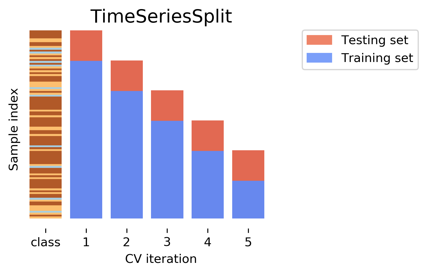
Temporal cross-validation with grid search

Below, we will show how to use temporal cross-validation to tune the hyperparameters of the random forest model. We will use TimeSeriesSplit from sklearn.model_selection to perform temporal cross-validation, which ensures that the training data is always before the validation data in time, thus avoiding data leakage.

from sklearn.model_selection import TimeSeriesSplit, GridSearchCV

# use only the training window for temporal CV to avoid leakage
tscv = TimeSeriesSplit(n_splits=5)

param_grid = {
  'max_depth': [None, 5, 10, 20],
  'min_samples_leaf': [1, 2, 4],
  'max_features': ['sqrt', 'log2', 0.5]
}

grid = GridSearchCV(
  estimator=RandomForestRegressor(random_state=42),
  param_grid=param_grid,
  cv=tscv,
  scoring='r2',
  n_jobs=-1,
  return_train_score=True
)

grid.fit(X_train, y_train)

print("Best hyperparameters (temporal CV):", grid.best_params_)
print(f"Best temporal CV R-squared: {grid.best_score_:.3f}")

# retrain on full training window with best params, evaluate on held-out test window
best_params = grid.best_params_
best_model = RandomForestRegressor(random_state=42, **best_params)
best_model.fit(X_train, y_train)

# r2 on training and testing data
train_r2_temporal = r2_score(y_train, best_model.predict(X_train))
print(f"Temporal split — Train R-squared with tuned params: {train_r2_temporal:.3f}")

test_r2_temporal = r2_score(y_test, best_model.predict(X_test))
print(f"Temporal split — Test R-squared with tuned params: {test_r2_temporal:.3f}")

Best hyperparameters (temporal CV): {'max_depth': 20, 'max_features': 0.5, 'min_samples_leaf': 1}
Best temporal CV R-squared: -0.269
Temporal split — Train R-squared with tuned params: 0.928
Temporal split — Test R-squared with tuned params: -2.687

The \(R^2\) on the training, testing, and cross-validated data are as follows:

Training data: 0.928
Testing data: -2.687
CV: -0.269

The hyperparameter tuning doesn’t improve the model performance on the testing data. This is due to insufficient data size and limited features. In practice, we would need more historical data (e.g. multiple years) and more potential relevant features (e.g. socio-economic, land use, historical fire incident density, remote sensing) to build a robust model for predicting daily LFB callouts.

Can you give it a try?

Future directions

That’s mostly for this practical. We have demonstrated how to predict LFB daily callouts withcross validation and hyperparameter tuning using grid search in both random and temporal data splits. The similar workflow can be applied to the classification task of predicting false alarms in fire incidents, and we will demonstrate this in later practicals.

References and recommendations:

There is not much (geospatial) machine learning research on London Fire Brigade datasets in academia. The blog by GTH Consulting provides some interesting articles on fire service data analysis in the UK, which receive lots of comments on LinkedIn (e.g. this).