Practical 2: Supervised learning framework and metrics
This week will introduce the supervised learning workflow using the use case of predicting daily callouts in London.
Learning Outcomes
You have familiarised yourself with the key steps in supervised machine learning workflow, including train-test split, cross validation, and hyperparameter tuning.
You are able to explain the differences between different workflows, including their pros and cons.
Starting the Practical
The process for every week will be the same: download the notebook to your DSSS folder (or wherever you keep your course materials), switch over to JupyterLab (which will be running in Podman/Docker) and get to work.
If you want to save the completed notebook to your Github repo, you can add, commit, and push the notebook in Git after you download it. When you’re done for the day, save your changes to the file (this is very important!), then add, commit, and push your work to save the completed notebook.
Note
Suggestions for a Better Learning Experience:
Set your operating system and software language to English: this will make it easier to follow tutorials, search for solutions online, and understand error messages.
Save all files to a cloud storage service: use platforms like Google Drive, OneDrive, Dropbox, or Git to ensure your work is backed up and can be restored easily when the laptop gets stolen or broken.
Avoid whitespace in file names and column names in datasets
London Fire Brigade Dataset
The London Fire Brigade (LFB) provides an open dataset containing information about multi-year fire incidents and fire engine moblisations in London. The fire incident dataset includes various details such as the location, time, and type of fire incidents, which can be useful for various analyses, including supervised learning tasks. The original dataset is available at here.
For convenience, we’ve processed and saved a subset of the LFB incident dataset in 2023 as LFB_2023_daily_data.csv (containing aggregated daily callouts in London) and LFB_2023_data.csv (containing individual incident information). The Python notebook for processing the original dataset is available here.
Key considerations
It is worthwhile reading the metadata before formatting a problem. The following are some key points to note:
The IncidentGroup column indicates the high-level incident type and consists of the following categories: False Alarm, Fire, Special Service. The ‘special service’ type refers to non-fire incidents, including assistance to other emergency services, such as helping with moving larger (i.e. bariatric) patients/people or rescuing people from lifts/elevators. The False Alarm type refers to fire callouts where no actual fire or emergency was present, and is further divided into three subtypes, including AFA, False alarm - Good intent, and False alarm - Malicious (see StopCodeDescription column). Obviously, if your research question is about fire incidents or fire risk, you should only focus on the Fire and False Alarm types in this column and remove Special Service type.
The location precision of incidents at Dwellings (i.e. residential buildings) is limited to the postcode district level (e.g. N2) for data privacy reasons. Therefore, the columns of Postcode_full, UPRN, Easting_m, Northing_m, Latitude, and Longitude are redacted or removed for Dwellings. This means that if you want to conduct geospatial analysis at a fine spatial resolution (e.g. building or street level), you should exclude incidents at Dwellings. If you want to conduct geospatial analysis for all incidents (including Dwellings), you should use spatial granularities coarser than postcode district level (e.g. boroughs, the whole London).
Stakeholders of fire service research
It is important to consider the potential stakeholders who might benefit from the insights derived from (geospatial) research of fire services. As far as I know, potential stakeholders include:
Local fire services including London Fire Brigade. Each fire service department has their data analyst and GIS team. They would be interested in understanding the patterns and trends of fire incidents to improve resource allocation, response times, and overall effectiveness of fire services. So far, the UK fire services don’t have lots of collaborations with academic researchers. If they need GIS expertise, they always outsource to private companies, such as Cadcorp and ORH.
National Fire Chiefs Council (NFCC, link). NFCC is a non-charity body representing Fire & Rescue Services at a national level and, as the professional voice of the fire and rescue service and aim for maximum impact. They strive to harness knowledge and expertise from across the country, bringing it together for the benefit of all.
Potential Use Cases
The LFB dataset can be used to formulate various supervised learning tasks:
Regression
Predicting daily LFB callouts in the whole London or each borough. Possible features include weather data, working day, public holiday, season, etc.
Time series forecasting of daily LFB callouts in the whole London or each borough using historical data. Possible features include historical callout data, weather data, working day, public holiday, season, etc.
Classification
Predicting whether a fire incident is a false alarm given the location available at the time of the callout, which includes time of day, day of week, postcode district, building type (dwelling or commercial).
etc.
Predicting daily LFB callouts
We will demonstrate how to formulate a regression problem to predict daily LFB callouts in London using weather and temporal features and how to compute the metrics for this problem. As we haven’t covered the workflow (e.g. train-test split, cross validation) of supervised learning or the algorithsm, we will use a basic workflow and the random forest algorithm.
# import data from https://raw.githubusercontent.com/huanfachen/DSSS_2025/refs/heads/main/data/LFB_2023_daily_data.csvimport pandas as pddf_lfb_daily = pd.read_csv("https://raw.githubusercontent.com/huanfachen/DSSS_2025/refs/heads/main/data/LFB_2023_daily_data.csv")print(df_lfb_daily.columns)
On the testing data, the RMSE is around 35.6, which means that the average prediction error is around 35.6 callouts per day. We can compare this RMSE with the mean daily callouts (around 346.5) to understand the relative size of the error, but this is not very useful as it does not consider the variance in daily callouts.
The R-squared on the testing data is around 0.18, which means that around 18% of the variance in daily callouts can be explained by the weather and temporal features used in the model. In comparison, the R-squared on the training data is around 0.92, which indicates that the model fits the training data well but does not generalise well to unseen data (i.e., overfitting).
This suggests that the model may need further tuning or that additional features may be needed to improve its predictive performance.
Predicting false alarm
We will now demonstrate how to formulate a classification problem that predicts if a callout to LFB is a actual fire or false alarm. As above, we will use a basic workflow and the random forest algorithm, and the focus here is to practice with different metrics for classification problems.
# import data from https://raw.githubusercontent.com/huanfachen/DSSS_2025/refs/heads/main/data/LFB_2023_data.csvimport pandas as pddf_lfb = pd.read_csv("https://raw.githubusercontent.com/huanfachen/DSSS_2025/refs/heads/main/data/LFB_2023_data.csv")# add DayOfWeek columndf_lfb['DayOfWeek'] = pd.to_datetime(df_lfb['DateOfCall']).dt.day_name()print(df_lfb.columns)
IncidentGroup
False Alarm        0.497899
Special Service    0.374637
Fire               0.127464
Name: proportion, dtype: float64
There are far more False Alarms (49.8%) than Fires (12.7%) in the dataset, which indicates class imbalance.
We will remove the Special Service type in the IncidentGroup column and formulate a binary classification problem to predict whether a callout is a false alarm (False Alarm) or an actual fire (Fire) using the following features available at the time of the callout:
Time of day (HourOfCall)
Day of week (DayOfWeek)
Building type (PropertyCategory).
As the Fire is a minority class, we will consider Fire as the positive class (1) and False Alarm as the negative class (0).
# import necessary librariesfrom sklearn.model_selection import train_test_splitfrom sklearn.ensemble import RandomForestClassifierfrom sklearn.metrics import accuracy_score, precision_score, recall_score, f1_score, confusion_matrixfrom sklearn.metrics import classification_report# remove 'Special Service' typedf_lfb = df_lfb[df_lfb['IncidentGroup'].isin(['False Alarm', 'Fire'])]# proportion of both classprint("proportion of Fire and False Alarm:")print(df_lfb['IncidentGroup'].value_counts(normalize=True))# prepare data for modelingfeature_cols = ['HourOfCall', 'DayOfWeek','PropertyCategory']X = df_lfb[feature_cols]# one-hot encode categorical featuresX = pd.get_dummies(X, columns=['DayOfWeek', 'PropertyCategory'], drop_first=True)y = df_lfb['IncidentGroup'].map({'False Alarm': 0, 'Fire': 1}) # map to binary labels# split data into training and testing setsX_train, X_test, y_train, y_test = train_test_split(X, y, test_size=0.2, random_state=42)# train Random Forest modelmodel = RandomForestClassifier(random_state=42)model.fit(X_train, y_train)# evaluate model performance on testing sety_pred = model.predict(X_test)accuracy = accuracy_score(y_test, y_pred)precision = precision_score(y_test, y_pred)recall = recall_score(y_test, y_pred)f1 = f1_score(y_test, y_pred)conf_matrix = confusion_matrix(y_test, y_pred)print(f'Accuracy: {accuracy:.3f}')print(f'Precision: {precision:.3f}')print(f'Recall: {recall:.3f}')print(f'F1-score: {f1:.3f}')# print classifcation reportprint(classification_report(y_test, y_pred, target_names=['False Alarm', 'Fire']))
proportion of Fire and False Alarm:
IncidentGroup
False Alarm 0.796176
Fire 0.203824
Name: proportion, dtype: float64
Accuracy: 0.881
Precision: 0.778
Recall: 0.569
F1-score: 0.657
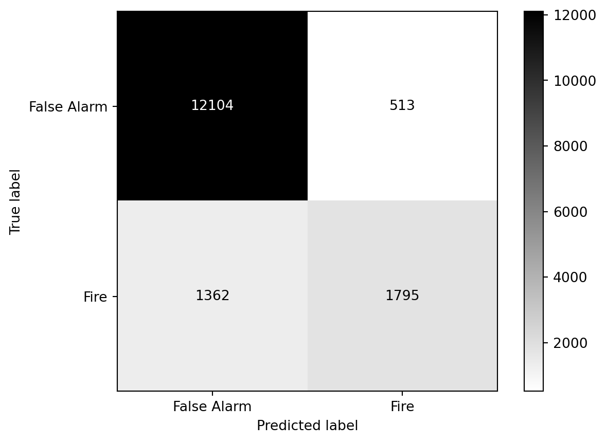
precision recall f1-score support
False Alarm 0.90 0.96 0.93 12617
Fire 0.78 0.57 0.66 3157
accuracy 0.88 15774
macro avg 0.84 0.76 0.79 15774
weighted avg 0.87 0.88 0.87 15774
# print the confusion matrix using ConfusionMatrixDisplayfrom sklearn.metrics import ConfusionMatrixDisplayConfusionMatrixDisplay(confusion_matrix=conf_matrix, display_labels=['False Alarm', 'Fire']).plot(cmap='gray_r')
Interpretation of metrics
As the target variable is highly imbalanced (79.6% False Alarm VS. 20.4% Fire), accuracy might not be a very useful metric here. A majority strategy that predicts everything as False Alarm would achieve an accuracy of around 0.796, which is similar to the accuracy of our RF model (around 0.881).
Considering recall and precision, which one is more reasonable for this task? In the fire service context, predicting a Fire as a False Alarm (i.e., false negative) is more serious than predicting a False Alarm as a Fire (i.e., false positive), as the former may lead to delayed response to actual fires. Therefore, we would like to predict all Fires correctly, in other words, maximising recall (or sensitivity). Therefore, recall is a more suitable metric than precision for this task.
To compare the performance and predictive power of our model against the majority strategy, the followign code is useful:
import numpy as npimport pandas as pd# majority strategy: predict everything as False Alarm (0)y_pred_majority = np.zeros_like(y_test)accuracy_majority = accuracy_score(y_test, y_pred_majority)precision_majority = precision_score(y_test, y_pred_majority, zero_division=0)recall_majority = recall_score(y_test, y_pred_majority)f1_majority = f1_score(y_test, y_pred_majority)# create a comparison tablecomparison_df = pd.DataFrame({'Model': ['Random Forest', 'Majority Strategy'],'Accuracy': [accuracy, accuracy_majority],'Precision': [precision, precision_majority],'Recall': [recall, recall_majority],'F1-score': [f1, f1_majority]})# limit the decimal places to 3print(comparison_df.round(3))
               Model  Accuracy  Precision  Recall  F1-score
0      Random Forest     0.881      0.778   0.569     0.657
1  Majority Strategy     0.800      0.000   0.000     0.000
The precision and recall of the majority strategy are both zero, which indicates that it has no predictive power for the minority class (i.e. Fire). In comparison, our RF model has a precision of around 0.778 and a recall of around 0.569.
Future directions
That’s mostly for this practical. In the following weeks, we will cover more details about supervised learning:
Meanwhile, for the above fire service research, we can include more features (e.g. land use, socio-economic, historical fire incident density, remote sensing) to improve the model performance.
References and recommendations:
There is not much (geospatial) machine learning research on London Fire Brigade datasets in academia. The blog by GTH Consulting provides some interesting articles on fire service data analysis in the UK, which receive lots of comments on LinkedIn (e.g. this).